
4. Bivariate Random variables
The real world involves interactions between forces, this is where we can start thinking about more than one thing going on at the same time. Much closer to reality. Single random variables are useful only for describing fairly simple problems, where the outcomes can be described by a single number. There are a number of reasons why we are interested in information that is more complex.
(1) most interesting problems do not involve simple averages like the average rainfall. We are more interested in the interactions of things, such as questions of relating rainfall with El Nino cycles. In this case we have a random variable for the possibilities for rainfall and one for the possibilities of water temperature in the Pacific. Other examples are endless, - e.g. not only if the patient is cured but also the age, sex, race and other characteristics of the patient. For this, we need to extend our ideas a little bit. - what is the relationship between age and success of a drug? - what is the relationship between income and schooling?
(2) The single distributions we have seen, namely the Bernoulli(p) and the normal, really only describe a single observation. In any type of learning from data we are likely to want to look at more than one observation. In statistics it turns out to be extremely helpful in checking what is going on and building up an understanding of the properties of, for example sample means, to consider each individual observation as an outcome from its own random variable, and so for more than one observation we have more than one random variable do deal with.
4.1 Bivariate Random Variables and Distributions
To start, we will be interested in having two random variables since this is the easiest case to consider. When we are comfortable with the two random variable world (so only two observations), then we can move on to the general problem of many random variables (and hence many observations).
In each case we are interested in probabilities on pairs of outcomes. Univariate : We have a Random Variable X, generated outcomes x, each with some probability of occuring. The Distribution for X was a way of capturing all of this information, i.e. in (x,p(x)). Bivariate We have two random Variables, X,Y generating outcome pairs (x,y). Each of these pairs has a probability of occurring . We can collect this information into { (x,y), P(x,y) } A JOINT DISTRIBUTION or BIVARIATE DISTRIBUTION would summarize this in the same way as the univariate distribution did above, but now in two dimensions.
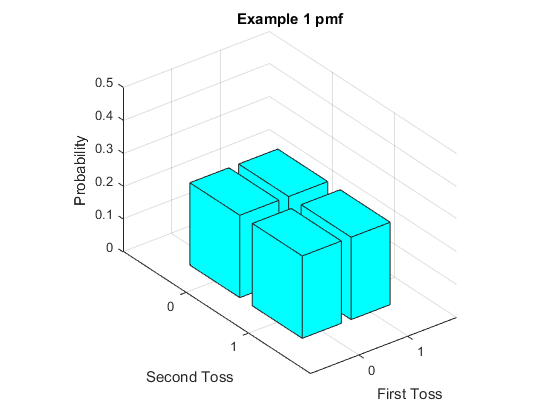
First Example: Toss two coins. This time we will describe the first toss by the random variable X and the second by Y. First toss $$ {X} = \begin{cases} 0 & \quad \text{Tails}\\ 1 & \quad \text{Heads }\\ \end{cases} $$ Second toss $$ {Y} = \begin{cases} 0 & \quad \text{Tails}\\ 1 & \quad \text{Heads }\\ \end{cases} $$
Thus each random variable by itself is a Bernoulli random variable. Notice that our Binomial S = X+Y and can be written as a function of these random variables. We can describe the joint probability distribution in a table
| Coin Toss Result | Random Variable Outcomes | Probability |
|---|---|---|
| Tail,Tail | (0,0) | $\frac{1}{4}$ |
| Tail, Head | (0,1) | $\frac{1}{4}$ |
| Head, Tail | (1,0) | $\frac{1}{4}$ |
| Head, Head | (1,1) | $\frac{1}{4}$ |
| sum=1 |
In the table we represent as numbers measured by the random variable pairs such as (0,0) which means (Tail,Tail) where the first element is the outcome fo the first toss and the second element is the outcome of the second toss. We have four pairs, which we assume are equally likely so by the Kolmogorov axioms (in particular so that the probabilities sum to one) we give each of the four equally likely outcomes a probability of one quarter.
We can draw a graph of the pmf for this bivariate random variable, although with more than one variable they are hard to read. With the heights of the boxes representing the probability, the graph is as follows.
It these discrete bivariate cases the following format is often clearer. Even though it does not nicely extend to situations where we have more than two random variables, it nicely brings out many of the concepts we will learn in this chapter.
| X\Y | 0 | 1 |
|---|---|---|
| 0 | $ \frac{1}{4} $ | $ \frac{1}{4} $ |
| 1 | $ \frac{1}{4} $ | $ \frac{1}{4} $ |
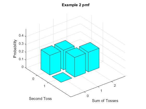
Example 2: Still two coin tosses but instead of measuring pairs $(X=x,Y=y) $ we will measure pairs ${S=s,Y=y} $ where S counts the number of Heads over both tosses (so in terms of last chapter, S=X+Y). So S can take values of zero (if we get two tails), one (if we get a tail then head or vice versa) or two (if we get two heads). Y is still the outcome on second toss (0=Tail, 1=Head). For this joint distribution, the table of outcomes is
| Coin Toss Result | Random Variable Outcomes | Probability |
|---|---|---|
| Tail,Tail | (0,0) | $\frac{1}{4}$ |
| Tail, Head | (1,1) | $\frac{1}{4}$ |
| Head, Tail | (1,0) | $\frac{1}{4}$ |
| Head, Head | (2,1) | $\frac{1}{4}$ |
| sum=1 |
(this is very similar to before, only the number assigning for S is different from that of X in the first example). Our distribution can now be written
| S\Y | 0 | 1 |
|---|---|---|
| 0 | $ \frac{1}{4} $ | 0 |
| 1 | $ \frac{1}{4} $ | $ \frac{1}{4} $ |
| 2 | 0 | $ \frac{1}{4} $ |
Drawn as a figure, we have the following graph.
In both these examples, the two bivariate random variables are derived from the same measurement (tossing two coins). How we choose to assign the numbers (choose the random variables) reflects merely the use we want to put the distribution to, i.e we cosntruct the random variables depending on what we want to learn or work with.
As with a single random variable, we can have continuous bivariate random variables as well. In this case the joint probability function takes the form $p(x,y)$, so now is a surface on the $x,y$ axes. It is just like the discrete bivariate random variable, and has all the properties we see with the discrete random variable, but now we replace summations over the $x,y$ space with integrals.
For example, consider the joint density function $$ p(x,y) = 6xy^2 $$ where $0 \le x \le 1$ and $0 \le y \le 1. $ We can picture this distribution in the figure below. As with the discrete problem, we have two base axes, one for $x$ and one for $y$. The height of the three dimensional curve is the joint probability.
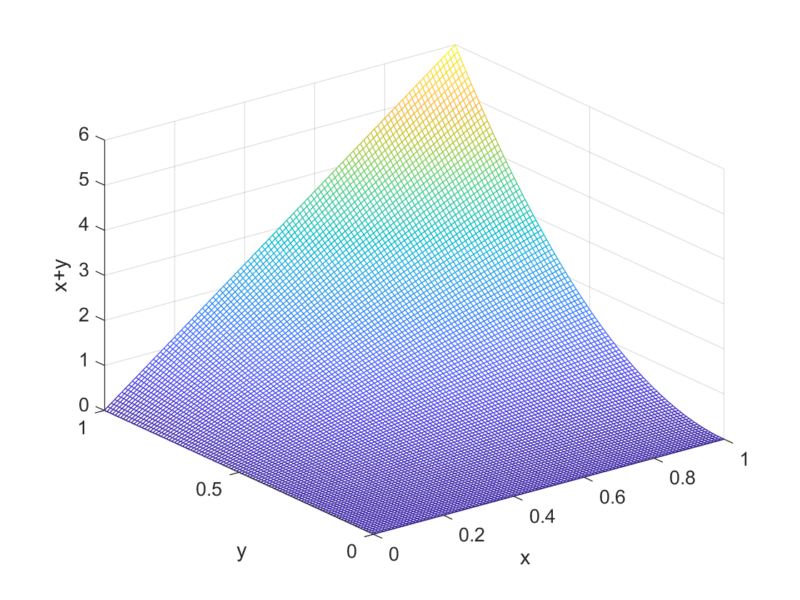
Probabilities are now integrals over areas inside the values for which we allow $x$ and $y$. In the figure they are areas under the three dimensional figure. For example if we want to compute the probability that $X \le \frac{1}{2}$ and $Y \le 1$ we would compute $$P(X \le \frac{1}{2},Y \le 1) = \int_{0}^{\frac{1}{2}} \int_0^1 6xy^2 dxdy. $$ Just integrate away (do this as an exercise) and you find that this is one quarter. All probabilities of events are constructed in this way with continuous random variables.
4.2 Marginal Distributions
Our joint distributions of the previous section contain all of the information in the distribution of $ X,Y $ or $ S $ individually. To see this, consider example one from above. When $ X=0 $, we have two possibilities for $ Y $, either the pair $(X=0,Y=0) $ or the pair $ (X=0,Y=1) $. Both of these possibilities are disjoint - which is to say that if one happens the other cannot. For disjoint events, the probability of one or the other happening is just the sum of the probabilities of each happening. In this case we have $$ P[X=0,Y=0]+P[X=0,Y=1]= \frac{1}{4} + \frac{1}{4} = \frac{1}{2} $$ We realize that this is the $ P[X=0] $. Basically, if we want to go from the joint distribution $ P[X=x,Y=y] $ to the distribution of $ X $ only, we need to remove the $ Y $ dimension information. To do so we simply add up the probabilites all the time we get $ X=0 $ over all of the possible combinations of $X=0 $ with any value for $ Y $.
We can see this easily by adding across the rows or down the columns in our table. For the first example we have
| X\Y | 0 | 1 | $ P[X=x]= $ |
|---|---|---|---|
| 0 | $ \frac{1}{4} $ | $ \frac{1}{4} $ | $ \frac{1}{2} $ |
| 1 | $ \frac{1}{4} $ | $ \frac{1}{4} $ | $ \frac{1}{2} $ |
| $ P[Y=y] = $ | $ \frac{1}{2} $ | $ \frac{1}{2} $ | sum = 1 |
Summing across the first row is just adding $ P[X=0,Y=0]+P[X=0,Y=1] $ which yeilds the correct probability for $ P[X=0] $ as we discussed in the first paragraph of this section. For the second row summing gives us $ P[X=1,Y=0]+P[X=1,Y=1] $ which again gives us one half, which we know is the correct answer for $ P[X=1] $. Similarly, summing down the columns gives us in the first column of probabilities $ P[X=0,Y=0]+P[X=1,Y=0] $ which is all the possibilities for when $ Y=0 $. Hence we obtain that the sum is $ P[Y=0] $. The same works for the second column of probabilities yeilding $ P[Y=1] $.
What we are doing is 'summing out the other dimension', for example to get $ P[X=x] $ from $ P[X=x,Y=y] $ we sum out the y part. The opposite is true for getting $ P[Y=y] $, we sum out the x part. So mathematically what we have is $$ P[X=x] = \sum_{\text{all y}} P[X=x,Y=y] $$ and $$ P[Y=y] = \sum_{\text{all x}} P[X=x,Y=y]. $$
It can get confusing now - once we have the joint distribution $ P[X=x,Y=y] $ we also have the distributions $ P[X=x] $ and $ P[Y=y] $. To be able to discuss clearly, we refer to the distributions $ P[X=x] $ and $ P[Y=y] $ as the marginal distribution of $ X$ and the marginal distribution of $ Y $ respectively. Marginal distributions always refer to the distribution of a single random variable.
Finally, notice that our Kolmogorov rule that the probabilities across all possibilities sum to one holds by definition. Since $ P[X=x,Y=y] $ is a distribution, the sum across all of the possible outcomes is one. When we sum out one dimension, we are left with the marginal distribution. When we sum out that dimension, we still get one, because doing these sums one after another is the same as summing over all the possibilties, which by definition sum to one. Mathematically this is just that $$\begin{equation} \begin{split} \sum_{\text{all (x,y) pairs}} P[X=x,Y=y] &= \sum_{\text{all x}} \sum_{\text{all y}} P[X=x,Y=y] \\ &= \sum_{\text{all x}} P[X=x] \\ &= 1. \end{split} \end{equation} $$
We can, for the second example see this in action. Before we start, realize that we know the marginal distributions for $ S $ and $ Y $. For $ S $, it is the sum of successes in two trials where the probability of a success (a Head) in each trial is $ p = \frac{1}{2} $. Hence the marginal distribution of $ S $ is the Binomial(2,$\frac{1}{2}$) distribution The marginal distribution for $ Y $ is as in example one, the usual distribution for a single coin toss. We also understand that for the second toss of the coin, that $ P(Y=0) = P(Y=1) = \frac{1}{2}$.
Now do this using the rules, building out the 'margins' of the distribution. We have
| S\Y | 0 | 1 | P(X=x)= |
|---|---|---|---|
| 0 | $ \frac{1}{4} $ | 0 | $ \frac{1}{4} $ |
| 1 | $ \frac{1}{4} $ | $ \frac{1}{4} $ | $ \frac{1}{2} $ |
| 2 | 0 | $ \frac{1}{4} $ | $ \frac{1}{4} $ |
| P(Y=y)= | $ \frac{1}{2}$ | $ \frac{1}{2} $ | sum = 1 |
We see indeed that our original marginal distributions are preserved.
For continuous distributions, the ideas are the same but now we use integrals instead of summations. To get the marginal distribution for $X$, we 'integrate out' in the direction of $Y$, and vice versa. We can do this with the example from the previous section, we have $$ p(x) = \int_0^1 6xy^2 dy = 6x \int_0^1 y^2 dy = 2x $$ and $$ p(y) = \int_0^1 6xy^2 dx = 6y^2 \int_0^1 x dx = 3y^2. $$ Note that the end points of the integrals are the lowest and highest values that $x$ and $y$ can take based on the definition of the density. You need to be careful with this. Finally, check for yourself that these really are probability distributions. To be so, they integrate to one.
4.3 Independence
The idea of independence is at once pretty obvious, and at the same time we still need to be careful. Independence simply means that with two random variables --- X and Y, that knowing the outcome of one of the random variables is entirely uninformative about the probabilities of the outcome of the second random variable. For example, suppose you are standing at the craps table. We could let the first random variable be the first throw of the dice, and the second random variable be the second throw of the dice. Now, suppose I told you that on the first throw a four was rolled. This does not help you understand the probabilities on the second throw --- they still have the same distribution we computed earlier in the course. Intuitively we understand this independence in terms of the rolls of the dice being 'unrelated'. What we will learn in this subsection is how this relates to distributions. The part at which we need to be careful arises when we think of this 'unrelatedness'. The formal definition of independence of two random variables, X and Y, is as follows. The random variables X and Y are independent if the joint distribution $$ P(X=x,Y=y) = P(X=x)P(Y=y) \text{ } \forall x,y.$$ We require that the joint distribution is the product of the marginal distributions for all possible outcomes. We determine whether or not this is true fairly quickly from the joint distribution tables.
Consider our first example. The table for the joint distribution and marginal distributions are repeated as follows.
| X\Y | 0 | 1 | $ P[X=x]= $ |
|---|---|---|---|
| 0 | $ \frac{1}{4} $ | $ \frac{1}{4} $ | $ \frac{1}{2} $ |
| 1 | $ \frac{1}{4} $ | $ \frac{1}{4} $ | $ \frac{1}{2} $ |
| $ P[Y=y] = $ | $ \frac{1}{2} $ | $ \frac{1}{2} $ | sum = 1 |
In this simple case for all $ (x,y)$ pairs the joint distribution has a probability of $\frac{1}{4}$ and the marginal distributions for $X$ and $Y$ have probabilities for all possible $x$ and $y$ equal to $ \frac{1}{2} $. So since $ \frac{1}{2}* \frac{1}{2} = \frac{1}{4} $ then for all possible $(x,y)$ we have that the formula $ P(X=x,Y=y) = P(X=x)P(Y=y)$ holds, and so here $X$ and $Y$ are independent. Note again that this relationship had to hold for every pair, if not the random variables would not be independent.
Now consider our second example. Again, the joint distribution of $ S,Y $ and the marginal distributions for each of the random variables are given in the table.
| S\Y | 0 | 1 | P[S=s]= |
|---|---|---|---|
| 0 | $ \frac{1}{4} $ | 0 | $ \frac{1}{4} $ |
| 1 | $ \frac{1}{4} $ | $ \frac{1}{4} $ | $ \frac{1}{2} $ |
| 2 | 0 | $ \frac{1}{4} $ | $ \frac{1}{4} $ |
| P[Y=y]= | $ \frac{1}{2} $ | $ \frac{1}{2} $ | sum = 1 |
Here the marginals for $ S $ are not the same, we simply check for each pair $(s,y)$. Consider first the middle row for $S$, i.e. when $S=1$. Here the $ P[S=1] = \frac{1}{2} $ and the marginal for Y has a probability of $ \frac{1}{2} $ for each outcome. The product of these is $ \frac{1}{4} $ for both otucomes for $ Y$, and indeed the joint distributions $ P[S=1,Y=y] = \frac{1}{4} = P[S=1]P[Y=y] $ for y=(0,1). For both of these cells of the table the indpendence requirement holds, but we recall that it must hold for all pairs. We quickly see that it does not hold for any of the other pairs. For example consider $ (S=0,Y=0) $. We have $ P[S=0,Y=0] = \frac{1}{4} $ however here $ P[S=0]*P[Y=0]= \frac{1}{4} * \frac{1}{4}= \frac{1}{8} $ and so the independence requirement does not hold for this cell. This means that the random variables $S$ and $Y$ are not independent.
To conclude that two random variables are not independent we only need to find one violation of the rule, then we can stop and conclude that the random variables are not indepdendent.
Hopefully the above two examples gave intuitively obvious results. For the first example, independence of the two coin flips is intuitively clear in the notion that the outcome from the first coin flip has no impact on the outcome for the second coin flip. In the second example, if you tell me $ S=2 $ I know that the outcome of the coin flipping exercise is that we saw two heads, so I know that $ Y=1 $. In this way there is a relationship between $S$ and $Y$.
For continuous distributions, the rule for independence is that the joint density is the product of the marginal densities for every possible $x$ and $y$. The words 'every possible' means ones that can actually happen, so you have to keep track of what values they can take. Mathematically we have $$ p(x,y) = p(x)p(y) $$ for independence.
In our example from the previous two sections, we have that $$ p(x,y) = 6xy^2 = (2x) (3y^2) = p(x)p(y) $$ and so indeed, our example is one where $X$ and $Y$ are independent. You might notice something here - we were able to factor the part involving $x$ from the part involving $y$, so each part is multiplies to get the joint density. Any time you can do that, we know the random variables are independent. For example if in the joint density there was an $x + y$, there is no way to factor that to being something in $x$ multiplied by something in $y$, and the random variables would then not be independent.
Independence of random variables plays a really important part in statistics. We will see in the end of this chapter and in the next chapter that having independent random variables makes a lot of the math much simpler. It is also a concept that is important when we come to thinking about collecting data, as we will see in Chapter 6.
4.4 Conditional Distributions
More information than just the marginal distributions is contained in the joint distribution. When we are interested in relationships between variables, we might be interested in the distribution of some outcome given a particular value of the other variable. For example we might have a joint distribution of income and education, but we are interested in the distribution of income given that someone completed college. If we had the joint distribution, we can work out these types of distributions. They are called conditional distributions because of this language - they are the distribution of one of the variables conditional on (i.e. given) the outcome of the other variable.
The formula for the conditional probability is given by $$ P[Y=y|X=x] = \frac{P[X=x,Y=y]}{P[X=x]} $$ We read $ P[Y=y|X=x] $ as the probability that $ Y=y $ conditional on (or given) that $ X=x$. We interpret it as the probability that we would see each value for $ y $ when we fix the outcome for $ X $ to be equal to $ x $.
Consider our example 2 from earlier, with the random variables $ S,Y $. First, consider what is really going on here. Just as we discussed in the previous subsection, if we know that $ S = 2 $ we know we saw two heads in the coin flip so we know that we had a hed on the second flip so we know that we must see $Y=1$ if $S=2$. Thus we should have that the probability of seeing a head on the second flip given we saw two heads is one. Mathematically we are saying that the $P[Y=1|S=2] = 1 $. We can apply our formula to see if this is so. We have that $$ P[Y=1|S=2] = \frac{P[S=2,Y=1]}{P[S=2]} = \frac{\frac{1}{4}}{\frac{1}{4}} = 1. $$ Naturally the other possibility for $Y$, i.e. $ Y=0 $ when $ S=2 $, cannot happen and must have a probability of zero. Again applying our formula, we see that this is indeed true. $$ P[Y=0|S=2] = \frac{P[S=2,Y=0]}{P[S=2]} = \frac{0}{\frac{1}{4}} = 0. $$ Choosing instead $ S=1 $, we know that if we know one of the tosses was a head (this is what $ S=1 $ is telling us) then it could have been that the tosses were either a Tail then a Head or vice versa. This means that $Y$ could be either zero or one. Indeed, if we just work this out intuitively, we realize that since all four outcomes from the two tosses (i.e. (Tail,Tail), (Tail, Head) etc.) have equal chance. If we narrow it down to (Tail,Head) and (Head,Tail) by conditioning on their being exactly one head over both tosses, then it seems reasonable that the probability that $Y=0$ and $ Y=1 $ are both the same. But since probabilities sum to one and these are the only two possibilities, this suggests that $P[Y=0|S=1] = P[Y=1|S=1] = \frac{1}{2} $. Again, we can apply our formulas. We have $$ P[Y=0|S=1] = \frac{P[S=1,Y=0]}{P[S=1]} = \frac{\frac{1}{4}}{\frac{1}{2}} = \frac{1}{2} $$ and $$ P[Y=1|S=1] = \frac{P[S=1,Y=1]}{P[S=1]} = \frac{\frac{1}{4}}{\frac{1}{2}} = \frac{1}{2} $$ so we obtain from the formula the expected results.
We realize at this point that the condition distribution is just another distribution, with the same properties as other distributions. Once we fix one of the random variables, we have a distribution in the random variable that is left. In the context of our example in example 2, this means that in addition to the marginal distribution for $Y$ we have three condtional distributions for $Y$, once for each value that can be taken on by $S$. For all of these distributions, marginal or conditional, the probability assignment must satisfy the Kolmogorov axioms. So all the distributions must have probabilities that sum to one.
That the conditional distributions need to sum to one gives intuition as to why the formula divides by the marginal distribution for the random variable we are conditioning on. This can be seen mathematically. We know that it must be that $ \sum_{\text{all y}} P[Y=y|X=x] = 1 $ since it is a distribution. But notice that $$\begin{equation} \begin{split} \sum_{\text{all y}}P[Y=y|X=x]&=\sum_{\text{all y}} \frac{P[X=x,Y=y]}{P[X=x]} \\ &= \frac{\sum_{\text{all y}} P[X=x,Y=y]}{P[X=x]} \\ &= \frac{P[X=x]}{P[X=x]} \\ &= 1. \end{split} \end{equation} $$ Hence dividing by $P[X=x]$ is exactly what we need to rebase that row of the distribution according to $X=x $ so that the probabilities sum to one.
We can also consider example 1 from earlier. For these random variables we have that in every case ($ x=0,1, y=0,1 $) that the joint probability $ P[X=x,Y=y] = \frac{1}{4} $ and that the marginals are all equal to one half. Hence for every pair of $ (x,y) $ we have that the conditional distribution $$ P[Y=y|X=x] = \frac{P[X=x,Y=y]}{P[X=x]} = \frac{\frac{1}{4}}{\frac{1}{2}} = \frac{1}{2}. $$ Consider what this means. We know that the marginal distribution for $ Y $ is $$ {Y} = \begin{cases} 0 & \quad \text{Tails}\\ 1 & \quad \text{Heads }\\ \end{cases} $$ But all of the condtinal distributions are the same as the marginal distribution. We have that $$ {Y|X=x} = \begin{cases} 0 & \quad \text{Tails}\\ 1 & \quad \text{Heads }\\ \end{cases} $$ So in this case conditioning on the first toss, meaning knowing the outcome of the first toss, tells us nothing about the distribution of $Y$. We have the same distribution whether or not we simply look at the marginal distribution for $Y$ and ignore $X$ as if we condition on seeing the outcome of $X$. That knowing the outcome from the first toss tells us nothing about the probabilities for the second toss sounds like the topic of the previous subsection, independence. This is another formulation of independence, namely two random variables $X$ and $Y$ are independent if $$ P[Y=y|X=x] = P[Y=y] $$ for all possible pairs of $(x,y) $. That this version of independence follows from our earlier one is straightforward, we have that $$\begin{equation} \begin{split} P[Y=y|X=x] = & \frac{P[X=x,Y=y]}{P[X=x]} \\ &= \frac{P[X=x]*P[Y=y]}{P[X=x]} \\ &= P[Y=y] \end{split} \end{equation} $$ where the second line follows only if $X$ and $Y$ are independent. This version of independence is much closer to how we really think about it. We say here that seeing the outcome of $X$ does not help us understand the probabilities over the outcomes for $Y$. Seeing a toss on the first coin does not help us understand the uncertainty of the outcome on the second coin. The two tosses are independent.
For continuous random variables, again the equations are very similar. It might seem that you cannot condition on a continuous random variable, because the probability of any particular value is zero and you cannot divide by zero for the formula. But this is not what happens - we divide by the marginal distribution. So the assumption is that the value of the marginal distribution is not zero, and recall that these distributions are not probabilities. So everything still works. We have then $$ p(y|x) = \frac{p(x,y)}{p(x)} $$ for all values where $p(x)>0$. This is the definition of the conditional probability for continuous random variables.
Note that this is still a distribution. This is to say that it is nonnegative - we can see that because the numerator and denominator are non negative. And it integrates to one when we integrate over the possible values for $Y$. You can see this too by realizing that $$ \begin{equation} \begin{split} \int p(y|x) dy = & \int \frac{p(x,y)}{p(x)} dy \\ &= \frac{\int p(x,y)dy}{p(x)} \\ &= \frac{p(x)}{p(x)} \\ &= 1. \end{split} \end{equation} $$ Notice this is almost identical in the steps as for the discrete case.
In both the discrete and the continuous case, a small reworking of the conditional distribution formula gives a formula for finding the joint probabilities from a conditional and a marginal one. In both cases we simply multiply both sides by the marginal distribution in the denominator of the right hand side. We have for the discrete case $$ P[X=x,Y=y] = P[X=x|Y=y] P[Y=y] $$ and for the continuous case $$ p(x,y) = p(x|y) p(y).$$ These types of manipulations come in handy for solving problems where we do not have the full joint distribution. This often happens when we have to estimate the probabilities from data, or build models.
An important understanding one should have is that in general $P[Y=y|X=x] \ne P[X=x|Y=y]$. This is to say that the probability of seeing a $Y$ outcome having seen an $X$ outcome is not the same as the reverse. Said this way it is obvious, but often when thinking casually we make this mistake. One thing you can take away from this course is to not make this mistake. For example, we might think that if a medical test for a rare disease has a 90% chance of being correct, that if we test positive for that disease there is a 90% chance we have it. But this is not correct.
We will set this up carefully with our two random variable math. Let $X$ be a 0-1 random variable where $X=1$ means that the test is positive, and zero for negative. Let $Y$ be the random variable, also 0-1, where $Y=1$ means we have the disease and zero means we do not. The real problem here is what do we really mean by "the test has 90% accuracy"? In English this is not a clear statement, we need to make it clear. A 90% chance of being correct could mean that $P[X=1|Y=1]=P[X=0|Y=0]=0.9$. In words, if we have the disease, the test will find that we have it with a probability of 0.9, if we do not have the disease the test will find that we do not have the disease with a probability of 0.9. So these are the two conditional probabilities, but they are not the conditional probability that we care about. We are (deathly) interested in the probability that we have the disease given that we tested positive for it, namely $P[Y=1|X=1]$, which is the reverse conditional probability.
How might we calculate this? If we had the entire joint distribution, we could simply use our conditional probability equation to compute this. But we are given some conditional probabilities. This is not enough to actually answer the question, but we can answer it with one more piece of information. Suppose that the incidence of the disease is $1/100$, it is a relatively rare disease. In math we are saying $P[Y=1]=1/100$. Without the test, this would be our chance of having the disease, but having tested positive we have more information. Our chance of having the disease is $P[Y=1|X=1]$, which we will now calculate.
We want to compute $$ P[Y=1|X=1] = \frac{P[X=1,Y=1]}{P[X=1]}. $$ Now we know that $P[X=1,Y=1] = P[X=1|Y=1]P[Y=1] = 0.9 * 0.01 = 0.009$. So this was easy. We also know from our marginal probability formula that $P[X=1] = P[X=1,Y=1] + P[X=1,Y=0]$. We already have the first term. The second term follows as we have $ P[X=1,Y=0] = P[X=1|Y=0]P[Y=0] = 0.1 * 0.99$ (because probabilities sum to one, and we have only two possibilities). So $P[X=1] = 0.9 * 0.01 + 0.1 * 0.99 = 0.108.$ Now we can compute the probability we want, we have $P[Y=1|X=1] = 9/108,$ slightly more than a 8% chance. Clearly not a 90% chance, as one might casually think.
Intuitively, the reason for this is that the base rate for the disease is small (which is what we mean by a rare disease). So even though the test has a 90% chance of getting it right, most of the mistakes are finding that healthy people have the disease, and very few of the mistakes are those with the disease having the disease missed by the test. So positives tend to be false positives for a rare disease, which is why doctors usually order more tests instead of telling you that you will die.
We can make this simpler using what is known as Baye's rule. Bayes rule is a rule that is constructed from the conditional probability rule, and gives a way of turning the conditional probabilty around. It is $$ P[Y=y|X=x] = P[X=x | Y=y] \frac{P[Y=y]}{P[X=x]}. $$ Now we see why the base rates, or the probabilities $P[Y=y],P[X=x]$ are important. If this ratio is not close to one, then the reversed conditional probability will be very different from the other way around. But this was exactly what happened in our example.
A deeper dive into conditional probabilities and the problems people have with understanding them is available here.
4.5 Functions of Two Random Variables
We are going to be interested in functions of random variables, and in particular the means and variances of functions of random variables. The next section discusses functions of random variables and the mean and variance. In particular we establish that even though when we take a function of random variables we obtain a new random variable, if we are only interested in the mean and variance of this new random variable we can work that out without working out the entire distribution of the new random variable. We then apply this idea to a the concept of the covariance.
In the last chapter we saw that if we take a function of a random variable, then we create a new random variable. Recall that, via the function, outcomes of the original random variable mapped to outcomes of the new random variable, and we simply brought across the probabilities to these new outcomes. We are also interested in mapping bivariate random variables to a new single random variable. There are many reasons to do this. Two examples are;
- Let $ X $ be a random variable describing earnings of person 1, $Y$ be a random variable describing earnings for person 2, and $ Z=((X+Y)/2)$ be the average earnings of the two people. Here $Z$ is a function of the other two random variables.
- Let $X$ be a random variable describing returns to a particular stock, $Y$ be a random variable describing earnings for another stock, we are interested in returns from the stock portfolio $W = aX + (1-a)Y$,where $ 0 \le a \le 1$ is the portfolio allocation to the first stock and is constant.
We will write our general formula as $ R=g(X,Y) $. So $R$ is a random variable built from the random variables $X,Y$. Following the same steps as in Section 3.8, we can construct a complete distribution for $R$. The first step would be to see what values $R$ would take on, these would be all $r=g(x,y)$ for all the pairs $(x,y)$. Then for each pair $(x,y)$ that mapped to a particular $r$, we would take the probabilities attached to each pair and carry them over to be the probability for that $r$. If more than one pair mapped to a particular $r$, we would add the probabilities together. Consider the first example from earlier in the chapter, and let R=X+Y. The distribution was
| X\Y | 0 | 1 |
|---|---|---|
| 0 | $ \frac{1}{4} $ | $ \frac{1}{4} $ |
| 1 | $ \frac{1}{4} $ | $ \frac{1}{4} $ |
The possible values for $R$ are now $(0,1,2)$ and the probabilities are given in the following table. We obtain this because we see that the pair $(0,0)$ is the only pair for $(x,y)$ that maps to $r=0$, and the probability of this pair is $\frac{1}{4} $ so this is the $ P[R=0] $. For $r=1$ we have that both the pairs $(0,1)$ and $(1,0)$ map to this outcome so we have that $ P[R=1] = \frac{1}{4}+ \frac{1}{4}= \frac{1}{2}.$ The final probability should be clear.
| R | P[R=r] |
|---|---|
| 0 | $ \frac{1}{4} $ |
| 1 | $ \frac{1}{2} $ |
| 2 | $ \frac{1}{4} $ |
We can now easily compute the mean of $R$, we have that $$\begin{equation} \begin{split} E[R] &= \sum_{\text{all r}} rP[R=r] \\ &= 0* \frac{1}{4} + 1* \frac{1}{2} +2* \frac{1}{4} \\ &= 1 \end{split} \end{equation} $$ (or we could notice that it is symmetric around one and hence the mean is one).
However we have another way to compute the mean here, without constructing the random variable $R$. Consider that $$ E[R] = \sum_{\text{all x}} \sum_{\text{all y}} (x+y)P[X=x,Y=y]. $$ That this gives the same answer follows from the way we constructed $R$, namely that each of the pairs mapped to $r$ and the probabilities carried across accordingly. Applying this formula to our example we have $$\begin{equation} \begin{split} E[R] &= \sum_{\text{all x}} \sum_{\text{all y}} (x+y)P[X=x,Y=y] \\ &= 0* \frac{1}{4} + 1* \frac{1}{4} + 1* \frac{1}{4} + 2* \frac{1}{4} \\ &= 1. \end{split} \end{equation} $$ Notice that the only difference was that in creating $R$ and then computing the mean is that the second and third terms of the second approach are put together, but the calculation is exactly the same in the end.
This is a general result, we have that for $R=g(X,Y)$ that $$\begin{equation} \begin{split} E[R] &= \sum_{\text{all r}} \sum_{\text{all y}} rP[R=r] \\ &= \sum_{\text{all x}} \sum_{\text{all y}} g(x,y)P[X=x,Y=y] \end{split} \end{equation} $$ The same idea can be used to construct the mean or variance of the function of random variables.
4.6 The Covariance
We now apply this idea of functions of a random variable to a the concept of the covariance, which is a special and useful function of two random variables.
An example of such a function of $X$ and $Y$ is the covariance. We have seen covariances before as a summary statistic calculated from data (just as we did for a mean) but there is an equivalent concept for a distribution (just as there is for a mean of a distribution). The covariance can be determined as $$ \sigma_{XY}=E(X-\mu_X)(Y-\mu_Y)P[X=x,Y=y] $$ This is a special case of the previous section where $ g(X,Y)=(X-\mu_X)(Y-\mu_Y) $
Consider the second example from this chapter. We can compute the correlation between $ S $ and $ Y $ by directly applying the formula using the joint distribution, we have that $$\begin{equation} \begin{split} E(S-\mu_S)(Y-\mu_Y) &= \sum_{\text{all s}} \sum_{\text{all y}}(s-\mu_S)(y-\mu_Y)P[S=s,Y=y] \\ \\ &= (0-1)(0-1/2)\frac{1}{4} +(1-1)∗(0-1/2)\frac{1}{4}+(1-1)(1-1/2)\frac{1}{4}+(2-1)(1-1/2)\frac{1}{4} \\ &= \frac{1}{8}+0+0+\frac{1}{8}=\frac{1}{4}. \end{split} \end{equation} $$
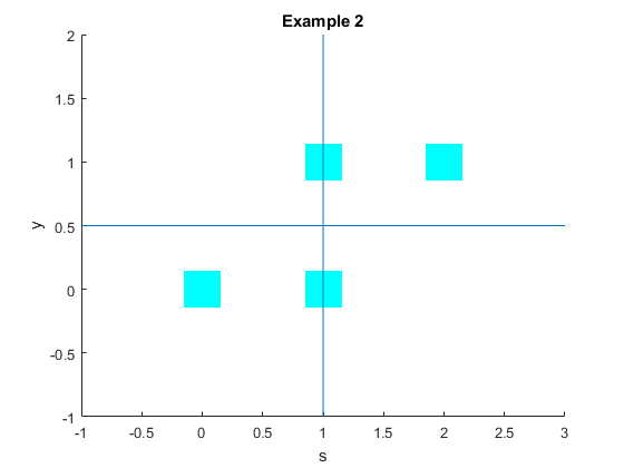
The covariance is positive here. As with the sample covariance, what matters here is the sign of the covariance, since the size of the covariance is affected by the units of measure. Here we have a positive covariance, indicating a positive relationship between $S$ and $Y$. This is not surprising. We have already noticed that seeing a large value for $S$, i.e. $S=2$ which is the only value above the mean, that this indicates that $Y$ will be above its mean with probability one. So a higher total count of heads is related (correlated) with a higher value for $Y$. This is what the positive covariance indicates. We can also think about this using the histogram of the probabilities, although for a bivariate random variable this is hard to draw in two dimensions.
The following figure shows the effect, where we have $S$ on the x axis and $Y$ on the y axis, think of the probabilities as being the height of the boxes (where the probabilities here are equal for each box). I have drawn lines at the mean of both $S$ and $Y$. We can see that the probabilities are overloaded in the North East and South West quadrants, giving the probabilities an upward sweep towards the right. Hence we get a positive covariance between the two random variables. Notice the analogy with how we did this with the data - the c concepts are different but clearly related.
If the probabilities are spread evenly over all four quadrants, then seeing X tells us nothing very interesting about Y. This is also the case that the covariance is close to zero. Mathematically what is happening is that we have (+ve*+ve) being cancelled by (+ve*-ve) terms etc.
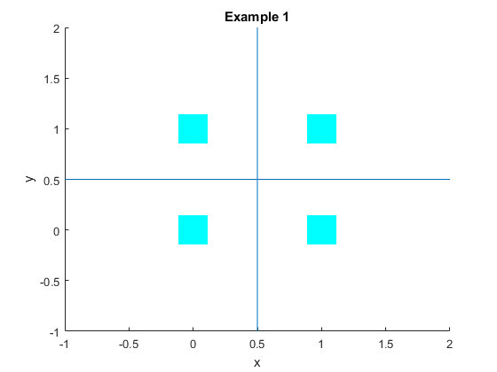
This was the situation in the first example for this chapter. Again working out the covariance we have that $$\begin{equation} \begin{split} E(X-\mu_X)(Y-\mu_Y) &= \sum_{\text{all x}} \sum_{\text{all y}}(x-\mu_X)(y-\mu_Y)P[X=x,Y=y] \\ \\ &= (0-\frac{1}{2})(0-\frac{1}{2})\frac{1}{4} +(1-\frac{1}{2})∗(0-\frac{1}{2})\frac{1}{4}+(0-\frac{1}{2})(1-\frac{1}{2})\frac{1}{4}+(1-\frac{1}{2})(1-\frac{1}{2})\frac{1}{4} \\ &= \frac{1}{16}-\frac{1}{16}-\frac{1}{16}+\frac{1}{16}=0. \end{split} \end{equation} $$Here the components of the covariance in the upper right and lower left quadrants exactly offset the components in the upper left and lower right. Hence we get a zero covariance. We already knew that $X$ and $Y$ here were independent, suggesting a link. It is always the case that independent random variables have a zero covariance. This is straightforward to show using our independence rule and the definition of the covariance.
In a picture we can see these offsets easily. We have $X$ on the x axis and $Y$ on the y axis, again think of the probabilities as being the height of the boxes (where the probabilities here are equal for each box). I have again drawn lines at the mean of both $X$ and $Y$. Here it is quite clear that there is an equal box in each quandrant, the two boxes in the North East and South West are offset by the boxes in the North West and South East. Hence we have no covariance between the two random variables $X$ and $Y$.
It is a general result that when two random variables are independent then their covariance is zero. This is something we can prove easily using our definition of independence. Suppose that two random variables, $X$ and $Y$, are independent, and recall that this means that $P[X=x,Y=y]=P[X=x]P[Y=y]$. The covariance is $$\begin{equation} \begin{split} \sigma_{XY} &= \sum_{\text{all x}} \sum_{\text{all y}}(x-\mu_X)(y-\mu_Y)P[X=x,Y=y] \\ &= \sum_{\text{all x}} \sum_{\text{all y}}(x-\mu_X)(y-\mu_Y)P[X=x]P[Y=y] \\ &= \sum_{\text{all x}} (x-\mu_X)P[X=x]\sum_{\text{all y}}(y-\mu_Y)P[Y=y] \\ &=0. \end{split} \end{equation} $$ The reason the last line is true is that $\sum_{\text{all x}} (x-\mu_X)P[X=x]=0$ and $\sum_{\text{all y}}(y-\mu_Y)P[Y=y]=0.$ So this always holds for independent random variables.
Unfortunately the converse is not true. It is possible that the covariance is zero but the two random variables are not independent.
As in the case of descriptive statistics, it is hard to get an idea from the raw number of the covariance as to how strong the relationship is. Thus we can also compute a correlation from the joint distribution (again this is a population concept, as opposed to a sample concept in the descriptive statistics).
The population correlation is given by $$ \rho_{XY}=\frac{\sigma_{XY}}{\sigma_{X}\sigma_{Y}}$$ where $\sigma_{X}$ is the standard deviation of $X$ and $\sigma_{Y}$ is the standard deviation of $Y$.
In terms of units, the numerator is X units times Y units but we divide by something in X units times something in Y units leaving the correlation unitless. As before, we have the properties
- The correlation has the same sign as the covariance so is interpretable in the same way
- $-1 \leq \rho_{XY} \leq 1$ so we can measure strength as distance from zero.
If we go to example 2, we have $$ \sigma_{S}=\sum_{s=0}^{2}(s-1)^2P[S=s]=(-1)^2\frac{1}{4}+(0)^2\frac{1}{2}+(1)^2\frac{1}{4}=\frac{1}{2} $$ and $$ \sigma_{Y}=\sum_{y=0}^{1}(s-\frac{1}{2})^2P[Y=y]=(-\frac{1}{2})^2\frac{1}{2}+(\frac{1}{2})^2\frac{1}{2}=\frac{1}{4} $$ so we have $$ \rho_{XY}=\frac{\frac{1}{4}}{\sqrt{1/2}\sqrt{1/4]}} \approx 0.71. $$ This is a fairly strong correlation, as we would expect from Figure 3 above.
4.7 Linear Combinations of Two Random Variables
We continue with taking functions of random variables. We now turn to linear combinations of random variables, and in particular the means and variances of linear combinations of two random variables. This sets us up for the next chapter, where we will be interested in taking linear combinations of many random variables.
We have for the general formula for the mean of $R$ when $R=g(X,Y)$ $$ E[R] = \sum_{\text{all r}} rP[R=r] $$ A function that we are particularly interested in is sums of random variables, i.e. $ g(X,Y)=X+Y. $ This is particularly important for understanding the random nature of sample means.
We can simply calculate the mean of the sum of two random variables, $$\begin{equation} \begin{split} E[X+Y]&= \sum_{\text{all x}} \sum_{\text{all y}}(x+y)P[X=x,Y=y] \\ &= \sum_{\text{all x}} \sum_{\text{all y}}xP[X=x,Y=y]+\sum_{\text{all x}} \sum_{\text{all y}}yP[X=x,Y=y] \\ &= \sum_{\text{all x}} x\sum_{\text{all y}}P[X=x,Y=y]+\sum_{\text{all y}} y\sum_{\text{all x}}P[X=x,Y=y] \\ &= \sum_{\text{all x}} x P[X=x]+\sum_{\text{all y}} y P[Y=y] \\ &=E[X]+E[Y]. \end{split} \end{equation} $$ So the general rule is that $E[X+Y]=E[X]+E[Y]$. Notice that this result holds for all random variables where the means exist, it does not depend on the distribution or correlation between the random variables. The reason that it works is in the proof above.
More generally we have the result $E[aX+bY]=aE[X]+bE[Y]$ for constants a and b. (see the box for a proof if you need, it is a very small variation around the result in the previous paragraph). A special case we are interested in in this course is when $a=b=\frac{1}{2}$, which gives us the sample mean. We have that $$ E\big[\frac{1}{2}X+\frac{1}{2}Y\big]=\frac{X+Y}{2} $$
Example : For the Binomial, we saw that if $S=X+Y$ when both $X$ and $Y$ are Bernoulli($p$) random variables, then the mean of $S$ is $2p$. This follows from the math above. We have that $E[X]=E[Y]=p$, so $E[S]=E[X]+E[Y]=p+p=2p$.
Since the sum of two (or more) random variables is itself a random variable, then it follows directly that these results extend to $E[aX+bY+cZ]=E[aX+bY]+cE[Z]=aE[X]+bE[Y]+cE[Z]$ where for the first step think of $aX+bY$ as a random variable. Alternatively you could take the formula at the start of this section and modify it slightly to show the result directly.
We are also interested in the variance of linear combinations of random variables. As with the mean, we can use our general formula and work from there. We have that $$\begin{equation} \begin{split} Var[X+Y]&=E[((X-\mu_{X})+(Y-\mu_{Y}))^2] \\ &= \sum_{\text{all x}} \sum_{\text{all y}}((x-\mu_{X})^2+(y-\mu_{Y})^2+2(x-\mu_{X})(y-\mu_{y}))P[X=x,Y=y] \\ &= \sum_{\text{all x}} \sum_{\text{all y}}(x-\mu_{X})^2P[X=x,Y=y]+\sum_{\text{all x}} \sum_{\text{all y}}(y-\mu_{Y})^2P[X=x,Y=y]\\ &+2\sum_{\text{all x}} \sum_{\text{all y}}(x-\mu_{X})^2(y-\mu_{Y})^2)P[X=x,Y=y] \\ &= \sum_{\text{all x}} (x-\mu_{X})^2\sum_{\text{all y}}P[X=x,Y=y]+\sum_{\text{all y}} (y-\mu_{Y})^2\sum_{\text{all x}}P[X=x,Y=y]+2\sigma_{XY} \\ &= \sum_{\text{all x}} (x-\mu_{X})^2 P[X=x]+\sum_{\text{all y}} (y-\mu_{Y})^2 P[Y=y]+2\sigma_{XY} \\ &=Var[X]+Var[Y]+2Cov(X,Y). \end{split} \end{equation} $$
This result extends to $$Var(aX+bY)=a^2Var(X)+b^2Var(Y)+2abCov(X,Y).$$ The proof again is a simple extension of the result above where the $a$ and $b$ simply float out to the front of each sum.
Finally, note a special case of this, when $X$ and $Y$ are independent. In this case the covariance as we have seen is zero, and so we have the result $Var(aX+bY)=a^2Var(X)+b^2Var(Y)$.
4.8 The Binomial Revisited
We turn our attention now to cleaning up some earlier handwaving. We talked about the Binomial distribution as the sum of indpendent Bernoulli distributions. Now we understand how to work with multiple random variables and understand independence, we can understand this more clearly.
For the binomial, we noted that it is the sum of $n$ independent Bernoulli(%p%) distributions. Let $n=2$. Then we have that the Binomial is simply $S=X+Y$. First notice that the outcomes match up. When we sum the random variables, we have possible outcomes $(0,1,2).$ But how about the probabilities? Suppose that the random variables $X$ and $Y$ are independent. Then we can write the marginal distributions (in tabular form) as
| X\Y | 0 | 1 | $ P[X=x]= $ |
|---|---|---|---|
| 0 | $ $ | $ $ | $ 1-p $ |
| 1 | $ $ | $ $ | $ p $ |
| $ P[Y=y] = $ | $ 1-p $ | $ p $ | sum = 1 |
Using the independence rule, we have that the joint probabilities $P[X=x,Y=y]=P[X=x]P[Y=y]$ so we can work out the empty entries in the table. We have
| X\Y | 0 | 1 | $ P[X=x]= $ |
|---|---|---|---|
| 0 | $ (1-p)^2 $ | $ p (1-p) $ | $ 1-p $ |
| 1 | $ p (1-p) $ | $ p ^2 $ | $ p $ |
| $ P[Y=y] = $ | $ 1-p $ | $ p $ | sum = 1 |
Now for S=X+Y we have the distribution
| S= | 0 | 1 | 2 |
|---|---|---|---|
| P[S=s] | $ (1-p)^2 $ | $ 2 p (1-p) $ | $ p^2 $ |
This is the Binomial $(n=2,p)$ distribution. The result extends for any $n$, but the tables get harder and harder to draw. Now there are two crucial assumptions here, (1) that the random variables are independent, and (2) that the random variables each have the same probability of success $p$. Without these two assumptions, we would not arrive at the Binomial probabilities!
To see the importance of the assumptions, lets relax the assumptions and see what happens. First, suppose that the random variables are not independent. The marginal distributions are as before, but now we cannot multiply them to get the joint probabilities. In my example we have the joint distribution
| X\Y | 0 | 1 | $ P[X=x]= $ |
|---|---|---|---|
| 0 | $ 1-p $ | $ 0 $ | $ 1-p $ |
| 1 | $ 0 $ | $ p $ | $ p $ |
| $ P[Y=y] = $ | $ 1-p $ | $ p $ | sum = 1 |
This is a valid joint density, and the marginal distributions are such that each of the random variables is still a Bernoulli($p$) random variable. What is happening is that they are not independent as in the discussion above (show that in fact they are perfectly dependent, knowing the outcome of one means you know the outcome of the other).
Now the distribution of $X+Y$ is as follows
| $X+Y$= | 0 | 1 | 2 |
|---|---|---|---|
| P[X+Y=x+y] | $ (1-p) $ | $ 0 $ | $ p $ |
This is clearly not the Binomial distribution.
The second problem was that we might not have the same probabilities of a success for each individual. Consider the marginal distributions in tabular form now as before but let the probability of a success be different for each random variable. We will assume that $X$ and $Y$ are independent, so obtain the joint probabilities as products of the marginals.
| X\Y | 0 | 1 | $ P[X=x]= $ |
|---|---|---|---|
| 0 | $ (1-p_x)(1-p_y) $ | $ p_y (1-p_x) $ | $ 1-p_x $ |
| 1 | $ p_x (1-p_y) $ | $ p_x p_y $ | $ p_x $ |
| $ P[Y=y] = $ | $ (1-p_y) $ | $ p_y $ | sum = 1 |
Now the probability of the sum $X+Y$ is
| $X+Y$= | 0 | 1 | 2 |
|---|---|---|---|
| P[X+Y=x+y]= | $ (1-p_x)(1-p_y) $ | $ p_y (1-p_x)+p_x (1-p_y) $ | $ p_x p_y $ |
This is again clearly not the Binomial distribution, unless $p_x = p_y$.
Copyright © Graham Elliott
Distributed By Themewagon