Worked Example for Bivariate Random Variables - Continuous RVs

This page works through all the ideas of Chapter 4 for a continuous bivariate random variable. Our $X,Y$ random variables have a probability distribution given by the following equation: $$ p(x,y) = x + y $$ for $0 \le x \le 1$ and $0\le y \le 1$.

So here our $X$ variable takes on values between zero and one, and our $Y$ variable takes on values between zero and one as well.

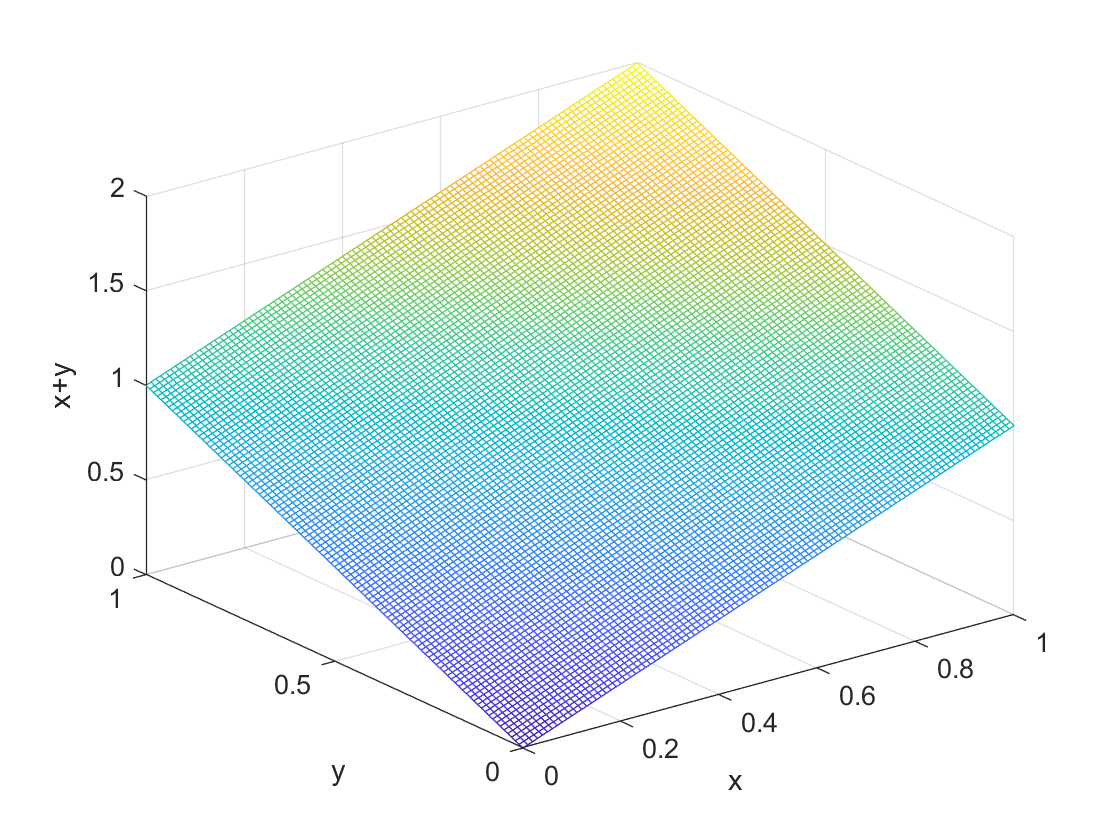
We can see what this probability density function looks like in the following figure. It is a three dimensional picture because now we have both $x$ and $y$ variables for the base of the figure and the surface shows the pdf $ p(x,y) = x + y $. It looks like a sheet of paper anchored at $(0,0)$ at zero, and at two when we get to $(1,1)$.

The probabilities are determined from the formula by intergrating over the formula, which are areas under the two dimensional curve in the above figure. The general formula for $P(a \le X \le b, c \le Y \le d)$ is $$ P(a \le X \le b, c \le Y \le d) = \int_a^b \int_c^d p(x,y) dxdy. $$ For example for the distribution above we could have $$ P(0 \le X \le 1/2, 0 \le Y \le 1/2) = \int_0^{1/2} \int_0^{1/2} (x+y) dxdy. $$ Solving is just standard integration. We have that $$\begin{equation} \begin{split} P(0 \le X \le 1/2, 0 \le Y \le 1/2)& = \int_0^{1/2} \int_0^{1/2} (x+y) dxdy \\ &= \int_0^{1/2} \int_0^{1/2}x dx dy + \int_0^{1/2} \int_0^{1/2} y dy dx\\ &= 2 \int_0^{1/2} \left[ \frac{x^2}{2} \right]_0^{1/2} dy \\ &= 1/8. \end{split} \end{equation} $$ Notice that in the third step I multiplied the integral for $x$ by 2 as both integrals are obviously equal to each other in the previous line.

From the joint distribution we can work out the marginal distributions using our formulas. We have that the distribution for $X$ is $$ p(x) = \int_0^1 (x+y)dy = x + \int_0^1 ydy = x + \frac{1}{2} $$ where we still have $0 \le x \le 1$. For the marginal distribution of $Y$ we integrate out the $x$ part so we have $$ p(y) = \int_0^1 (x+y)dx = y + \int_0^1 xdx = y + \frac{1}{2}. $$ That they are the same is not so surprising given the symmetry of the problem.

We can work out the means etc. of these distributions as well. We have $$ EX = \int_0^1 x (x+\frac{1}{2})dx = \int_0^1 x^2dx + \frac{1}{2}\int_0^1 xdx = \frac{7}{12} $$ The mean of $Y$ is obviously the same.

For the conditional distribution of $Y$ given $X$, it is again we need to use the general formula. We have in general $$ p(y|x) = \frac{p(x,y)}{p(x)} $$ and in our example $$ p(y|x) = \frac{x+y}{x+\frac{1}{2}}. $$ Notice that this is a distribution over possible values for $x$, so the values it can take are for $0 \le x \le 1$.

We can consider whether or not $X$ and $Y$ are independent. They are independent if the conditional distribution is equal to the marginal distribution.

The conditional mean of $Y$ as a function of $X$ follows from computing the mean using the conditional distribution probability function, we have $$ E[Y|X] = \int_0^1 y p(y|x) dy $$ in general. For our example this is $$ E[Y|X] = \int_0^1 y \frac{x+y}{x+\frac{1}{2}} dy = \frac{2+3x}{3+6x}. $$ This is clearly different from the marginal distribution for $Y$ we computed above. So we can conclude that the random variables are not independent.

We can picture the relationship between the variables by drawing the graph of the conditional mean against $x$. This is shown in the following figure. We see that the conditional mean is decreasing in $x$. We read this as a larger $x$ is associated with a smaller $y$, in the sense that the mean of $Y$ is smaller. We can think of why tracing out the conditional mean might be useful in practice. We can think of the conditional mean as a 'forecast' of $Y$ when we know $x$. We could also think about this as being the effect of $x$ on $Y$ (although you will see in later courses this is hard to justify sometimes). Later you will learn about a technique known as regression - Regression is basically a statistical approach to trace out the relationship between the conditional mean and an $x$ that relates to $Y$. This could be linear regression, or as in our example trying to find a nonlinear function (which is basically what machine learning is trying to do with numerical data.)

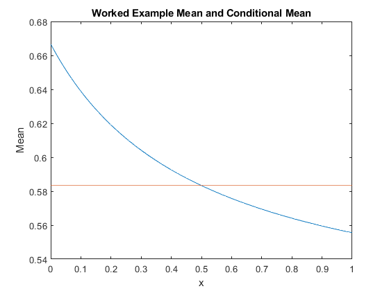
We can also see, looking at the figure, why the conditional mean might be more useful than the mean (which is denoted by the flat line in the figure above). For example suppose that the $x$ variable is an index of the wealth of your customer, and the $y$ variable is an index of how much the customers spend in your store (the indexes are normalized to zero to one). Then knowing that a random customer spends on average at $7/12$ on the index is useful, but it is far more useful to know that the wealthier ones spend less on average than the poorer ones. You know much more about how your customers spend, and can target this accordingly.