3. Probability Distributions
So we worked in the last chapter with data, creating sample distributions (we use the word sample here to denote that it is the distribution that came with data) and sample moments (such as the mean or the standard deviation again from data). But recall what we really want to do. We want to be able to relate data to what our theories suggest data to be. In order to do this, we need to be able to work out similar objects to those we computed with data but come from our theories. We take the first step towards this in this chapter. This chapter develops the use of probability theory to provide a description of what our theory suggests. If you want more background than we cover in the chapter, see Probability Basics .
"The most important questions of life are, for the most part, really only problems of probability." Pierre Simon de Laplace, "Theorie Analytique des Probabilites"
3.1 Discrete Random Variables
Random variables describe our uncertainty over what might happen. Suppose we want to measure the speed of light. Our theory might say it is a fixed number, but taking into account measurement error we might expect other values near that number. So the outcome of any measurement has some uncertainty. Alternatively, if we are measuring the unemployment rate, a particular person is either employed or not. However before taking the measurement (asking them, say in a survey) we do not know the outcome. Random variables describe the uncertainty in these measurements. When we are uncertain as to what might happen, we are left to describe both
(a) the types of outcomes possible
(b) the relative importance of taking each possible outcome seriously.
Example 1 (toss a coin).
When we go to toss a coin, we can easily evaluate the possible outcomes. They are that we get a Head or a Tail. Before tossing the coin, we do not know which will occur, but we know we are limited to one or the other. We refer to the possibilities as 'outcomes', and will denote them by lower case letters from the alphabet. We could for example set $$ {x} = \begin{cases} \text{Tails} & \quad \text{}\\ \text{Heads} & \quad \text{ }\\ \end{cases} $$ However, it turns out to be a lot easier to use numbers instead of words to record outcomes and work with them (think of computing the average). Hence we usually set (for a two outcome problem like this) the outcomes to be $$ {x} = \begin{cases} 0 & \quad \text{Tails}\\ 1 & \quad \text{Heads }\\ \end{cases} $$ so x can take one of two numbers (since there are just two outcomes).
Example 2. (toss a pair of dice). Here the outcomes are a bit complicated, and we might want to think about what we really want to use the result for. For example we could collect all pairs, say the number on the first die and the number on the second die. This would be outcomes of the form (3,4) for for a three on the first die and a four on the second die for example. Or we might be interested only in the sum of the two values (say when you are playing craps), in which case we have outcomes from 2 (if the dice both show a 1) to 12 (if both show a six), i.e. x can take on any integer value from 2 to 12.
After understanding what types of outcomes are possible, the next useful thing to do is work out which of the outcomes are more worthy of attention and which are less interesting. To do this, we attach a probability to each outcome. Most of us have a feel for what we mean by probability or the chance that something happens. We are used to using this term, basically correctly, in everyday conversation. This tool --- of being able to think of our not knowing what may happen by examining not just what could happen but also how likely each of these things are --- is incredibly useful. What exactly is a probability? The usual way to think about probabilities for events is to consider them as frequencies of observing that event in many repetitions. e.g. We assign a probability of one half to the chance of a Head in a toss of a fair coin because if we did it many many times this is the percentage of times we would see a Head appear in very many tosses. (put graph of this phenomena here, also maybe talk about the guy in WWII who checked it). This is a little conceptually unclear as many things we would like to assign probabilities to cannot be repeated. e.g. What is the probability that you will become a multi millionaire in your life? Unless you are a Bhuddist life is a one-shot deal, but we still may want to place a probability on this (can always think of parrallel universes). Finally, probabilites can be thought of as 'fair bets'. This would be a bet you are willing to take both sides of. We tend to avoid these philosophical issues by simply allowing any probability so long as it makes 'sense'. By this we mean that it satisfies certain rules, including (a) probabilities must be nonnegative. (b) probabilities of 'disjoint' possibilities can be summed to get total probability, (b) the probability of something that must happen is equal to one. These are known as the Kolmogorov axioms.
Example 1 (coin toss). If we think of the frequency rule, then the proportion of heads to total tosses can be zero or one (two headed coin), or some number in between. It cannot be negative, since we cannot get a negative number of heads in any amount of tosses. Further, the probability of either a head or a tail must be one, since one of these must appear. But what is the probability of a head when we toss a coin? If the coin is fair, we think of it as equal to one half, which is to say that there is an even chance of a head or a tail. Hence we would usually be happy writing the probabilities as
P[head]=1/2
P[Tail]=1/2.
This we can most likely agree on.
Example 2. (toss two dice, add the values). In this case we can also appeal to fairness to try and work out what probabilites to assign. First, notice that with 6 possible values on each die, there are 36 possible combinations in total. If each has the same chance of happening, we are comfortable giving the probability of 1/36 for each possible pair. Now we can work out the probabilities for each sum, by adding up how many times each can occur. For example we can only get $x=2$ one possible way, if both faces show a one. Hence we would give this a probability of 1/36. For $x=3$ we have two possible ways of getting this, the first face could be one and the second face equal to 2 or vice versa. Hence we give this outcome a probability of 2/36. Continuing in this way we can give values to all of the possibilities. Note that the probabilities will sum to one, so our axioms will hold in this accounting exercise.
The entire scenario, which is to say (a) the description of how we define the numbers (b) the collection of possible outcomes (c) the probabilities we give to the outcomes is known collectively as a Random Variable, which we denote somewhat obscurely by an upper case letter from the alphabet. Example 1 (coin toss). We have (a) description: toss a coin, let Heads equal one and tails equal zero (b) x=1,x=0 (c) P(Head)=P(Tail)=1/2 is the random variable X. Notice that our usual notation/terminology is that X has outcomes x=0,x=1 and P[X=0]=1/2. P[X=1]=1/2. The use of the X is just to save writing down the whole description over and over again, which is very helpful for complicated descriptions. As you might guess we also have math for random variables, so it is useful to have it like a mathematical symbol. Example 2. (toss two dice, add total). Here X denotes (a) toss two fair dice, count total value for the outcome (b) x=2,3,...,12. (c) P[X=2]=1/36, ... Again, when I say 'the random variable measuring the total on two dice' or X I mean the same thing, which is all this information together. Probabilities and multiple outcomes Can I always just add probabilities like we have been? Example 1: $P(X=1 or X=0) = P(X=1)+P(X=0)=1/2 + 1/2 =1$. Example 2.(a) To get P(X=3) we added Probability that we had (1,2) and (2,1) to get 2/36. (b) $P(X<=7)=P(X=1)+...+P(X=7)=21/36$ $P(X>=7)=P(X=7)+....+P(X=12)=21/36.$ The answer is no. Consider these two probabilities. P(X>=7)+P(X<=7)= 42/36 > 1. But we cannot have a probability of greater than one. What happenned is that we double counted. Here we double counted P(X=7). If we break up the problem into its 'nonoverlapping' parts, then we get the correct answer. In practice this is exactly what we will do --- in the probability models we construct we have the outcomes in their basic parts and so we do not usually run into problems. Finally, this section was called 'discrete' random variables. What makes these discrete is that we are able to count the number of outcomes. In example one there are 2 outcomes, in example three there are 11 outcomes. As we will see later sometimes we cannot count the outcomes, but for now we will continue to work with discrete random variables.
"While writing my book [Stochastic Processes] I had an argument with Feller. He asserted that everyone said ``random variable'' and I asserted that everyone said ``chance variable.'' We obviously had to use the same name in our books, so we decided the issue by a stochastic procedure. That is, we tossed for it and he won." J. Doob (a famous probabilist), From the magazine Statistical Science, on how the name 'random variables' came to be.
3.2 Probability Distributions
We just saw the first step in constructing mathematical models for our theories. We converted everything to numbers because they are easy to work with. Now we turn to keeping track of all the information in the random variables and the probabilities attached to each possibility.
The collection of the outcomes and the probabilities together is known as a Probability Distribution. We can collect them together by either
- Table
- Graph; or
- Formula
The particular form does not matter, it is all about convenience with the numbers to compute what we need to compute. When there are many outcomes, tables become cumbersome so we switch to formulas. For visualizing the distribution, the graph is going to be the most useful. Example 1 (Coin Toss). We have already put it in a Table, this would be
| $X$ | $P(X=x)$ |
|---|---|
| 0 | $ \frac{1}{2}$ |
| 1 | $ \frac{1}{2}$ |
In a graph it is simply
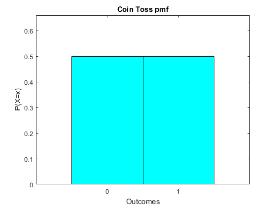
The formula is straightforward, $P[X=x]=0.5, x=0,1$. We call such a plot of the outcomes and probabilities a Probability Mass Function. It is a simple way to express the information in the table.
Example 2 (2 dice, sum total) Again, we can put this in a Table. It is
| $X$ | $ P(X=x) $ |
|---|---|
| 2 | $ \frac{1}{36}$ |
| 3 | $ \frac{2}{36}$ |
| 4 | $ \frac{3}{36}$ |
| 5 | $ \frac{4}{36}$ |
| 6 | $ \frac{5}{36}$ |
| 7 | $ \frac{6}{36}$ |
| 8 | $ \frac{5}{36}$ |
| 9 | $ \frac{4}{36}$ |
| 10 | $ \frac{3}{36}$ |
| 11 | $ \frac{2}{36}$ |
| 12 | $ \frac{1}{36}$ |
In a graph it is
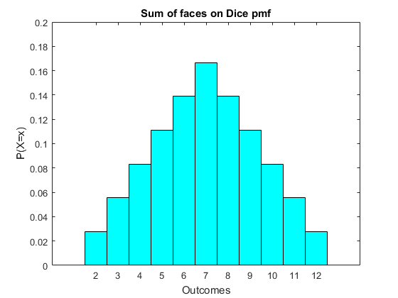
We can write this as a formula, it is $$ P(X=x) = \begin{cases} \frac{x-1}{36} & \quad \text{if } x \le 7\\ \frac{13-x}{36} & \quad \text{if } x >7 \\ \end{cases} $$ Notice that the graph allows simple visual understandings of the chances of each outcome at the craps table. The pmf is symmetric.
We refer to the random variables for each of our two examples as discrete random variables because there are a finite number of values that X can take on. In example 1 there are two possible values, for example 2 there are 11 possible values. The probability distributions (graphs of x against $\text{P}(X=x)$ are known as probability mass functions. We typically abbreviate this to pmf.
These probability mass functions look similar to our histograms when we were working with data. Indeed, this is our first view of how we might relate our theories, described by a pmf, with our data described in a histogram. Suppose we tossed a coin 100 times, and drew the histogram of our results using zero for a Tail and one for a Head. The frequency histogram should look like our pmf for the coin toss example. If it did, then we would be sure our theoretical model of coin tossing is correct. If it looked different, we would have something to explain.
The pmf is a great tool, one we will see again and again. In part for mathematical reasons, statisticians also like to work with the cumulative version of this. Just like the cumulative version of a histogram, we add up all the probabilities below each x. Mathematically we have $$ P(X \le x) = \sum_{y=-\infty}^{x} P(X=y) $$ We refer to this as the cumulative density function (denoted cdf). This too looks familiar from our data analysis, it corresponds with our empirical cdf (hence the similar name). Again, if our theory suggests a cdf of a certain form, our empirical cdf should look similar if our theory is correct.
For example 1, our cdf is quite trivial. In a graph it is as follows.
For example 2 it is a little more involved, see the following graph
In a table, for example 2 we have the following pmf and cdf
| $X$ | $ P(X=x) $ | $ P(X \le x) $ |
|---|---|---|
| 2 | $ \frac{1}{36}$ | $ \frac{1}{36}$ |
| 3 | $ \frac{2}{36}$ | $ \frac{3}{36}$ |
| 4 | $ \frac{3}{36}$ | $ \frac{6}{36}$ |
| 5 | $ \frac{4}{36}$ | $ \frac{10}{36}$ |
| 6 | $ \frac{5}{36}$ | $ \frac{15}{36}$ |
| 7 | $ \frac{6}{36}$ | $ \frac{21}{36}$ |
| 8 | $ \frac{5}{36}$ | $ \frac{26}{36}$ |
| 9 | $ \frac{4}{36}$ | $ \frac{30}{36}$ |
| 10 | $ \frac{3}{36}$ | $ \frac{33}{36}$ |
| 11 | $ \frac{2}{36}$ | $ \frac{35}{36}$ |
| 12 | $ \frac{1}{36}$ | $ \frac{36}{36}=1$ |
From the pmf or cdf we can do simple calculations. Notice that for all of our x′s, if one happens the other cannot. This means that we do not have to worry about overlap when we add probabilities.
e.g. Craps. Craps is a gambling game based on the outcome of the sum of the faces of two dice. Rules: Come out roll rolling a 2,3 of 12 looses the stake, a 7 or 11 wins. Other rolls lead to the game continuing with that number becoming point. On the point, rolling a 7 looses (this is called craps). See Box X for more information.
- What is the chance you loose your stake on the comeout roll? This is $\text{P[roll a } 2,3 \text{ or } 12]=(1+2+1)/36=4/36$.
- What is the chance that you double your stake on the come out roll? This is $\text{P[roll a } 7,11] = (6+2)/36=8/36$.
- What is the chance you go the the point? This is what remains, it is $1-12/36=24/36=2/3$.
We can write the distribution for the two dice problem as a formula, it is $$ P(X=x) = \begin{cases} \frac{x-1}{36} & \quad \text{if } x \le 7\\ \frac{13-x}{36} & \quad \text{if } x >7 \\ \end{cases} $$ Notice that the graph allows simple visual understandings of the chances of each outcome at the craps table. The PMF is symmetric.
We refer to the random variables for each of our two examples as discrete random variables because there are a finite number of values that X can take on. In example 1 there are two possible values, for example 2 there are 11 possible values. The probability distributions (graphs of x against $\text{P}(X=x)$ are known as probability mass functions. We typically abbreviate this to pmf.
These probability mass functions look similar to our histograms when we were working with data. Indeed, this is our first view of how we might relate our theories, described by a pmf, with our data described in a histogram. Suppose we tossed a coin 100 times, and drew the histogram of our results using zero for a Tail and one for a Head. The frequency histogram should look like our pmf for the coin toss example. If it did, then we would be sure our theoretical model of coin tossing is correct. If it looked different, we would have something to explain.
3.3 Population Moments
We do not have to work always with the whole distribution. Sometimes we are interested in the moments of the distributions
We can also calculate summary statistics of the distribution. What number would you expect to see if you had one draw from the distribution? By draw I mean that you got to see one outcome only. This would for our examples be Example 1: Toss a coin once, what outcome would I expect to see? Example 2: Toss two dice, add the values. What outcome would I expect to see? Lets look at the distributions and see what we mean here. What would be a good 'measure of location' of the random variable outcomes? The balance point of the pmf might spring to mind. For this problem, example 2 is easier to examine first.
In example 2, the pmf is symmetric, so the balancing point must be in the center. This is a value of x=7, i.e the roll we definitely never want (unless it is the come out roll)! No surprise that the casinos want that outcome for themselves. In example 1 it is not so clear, since both possible outcomes happen with the same frequency. By the balance point analogy, we would expect a value of one half, which never even happens. How might we compute the mean? We could think of the possible outcomes and use the formula we used for the sample. i.e. we have the following for example one.
| $X$ | $P(X=x)$ |
|---|---|
| 0 | $ \frac{1}{2}$ |
| 1 | $ \frac{1}{2}$ |
Our formula for data would be to compute the mean as $ 0* \frac{1}{2} + 1*\frac{1}{2} =\frac{1}{2}. $ This is clearly the balancing point.
For example 2, we can also take this approach. We have here 36 equally likely outcomes, think of this as 36 datapoints. What happens if we thought of this as data? The formula would be $$ \frac{1}{36}*2+\frac{2}{36}*3+\frac{3}{36}*4+\frac{4}{36}*5+\frac{5}{36}*6+\frac{6}{36}*7 $$ $$+\frac{5}{36}*8+\frac{4}{36}*9+\frac{3}{36}*10+\frac{2}{36}*11+\frac{1}{36}*12 = \frac{252}{36} = 7 $$ This is clearly the answer we were expecting. In both calculations we obtain a result that looks like the balancing point of the pmf
We will denote the population mean of a distribution as $\mu $. For a discrete random variable the formula for the population mean is $$ \mu = \sum_{x} x P(X=x) $$ We will drop the 'population' or 'sample' and simply say mean when we know which one of these we are talking about. You do need to keep clear the distinction between the sample mean and population mean however, as from Chapter 7 we will see them both in the same formula.
Thinking again to relating our data to our theory, the sample mean will be our data measurement that corresponds to our population mean which is our theoretical concept. Clearly for a theory to be reasonable the sample mean will have to be near the population mean. They won't be the same however, they just need to be close enough. We need to develop a bit of math before we can understand what 'close enough' actually means.
It might be confusing that we have the same name 'mean' for two different things, but of course we have seen that they are related. We have another name for the population mean, we call it the 'Expected Value of X'. Above I used these exact words to describe the population mean, it is the value we might expect to see or see most often. So calling it the expected value makes a lot of sense. In practice the mean is just one example of an expected value, the Expectation Operator is defined in the following way. If we have a random variable X, and suppose we take some function of X, f(X). Then the expectation operator is defined as $$ \text{E[f(X)]} = \sum_{x} f(x) P(X=x). $$ The mean is a special case where f(X)=X (compare the formulas for E[X] and for $\mu$ above).
Just like with the mean, we have a population variance as well. Recall that the variance looked at the squared distance of the outcomes from the mean. Analogously with the sample version, we define the population variance to be $$ \sigma^{2} = \sum_{x} (x-\mu)^2 P(X=x). $$ Notice that this is just a special case of the expectation operator above where we have set $ f(x)=(x-\mu)^2.$ Because the variance plays such a huge role in statistics we give it it's own special letter. We refer to the positive square root of the variance as the standard deviation, denoted $\sigma$, and so the variance is $\sigma^2$.
In practice computing the variance is just simply applying the formula. For the coin toss example, we have that the variance is $$\begin{equation} \begin{split} \sigma^{2} &= \sum_{x} (x-\mu)^2 P(X=x) \\ &= (0 - \frac{1}{2} )^2 \frac{1}{2} + (1 - \frac{1}{2} )^2 \frac{1}{2} \\ &= \frac{1}{8} + \frac{1}{8} \\ &= \frac{1}{4} \end{split} \end{equation} $$
A worked example for a discrete random variable is available here.
3.4 The Bernoulli Distribution
Some distributions are so useful and ubiquitous that it will help to understand them well. The first and simplest of the general distributions is the Bernoulli distribution
The first of these relates to situations where there are only two outcomes, like our toss of a coin. Practical (real) examples include
- Does a drug or operating procedure cure the patient?
- Will you vote for the incumbant party?
- Will you buy my product?
- Did you get a job in the six months after graduating?
- Did the stock market go up today?
- Did it rain today?
All of these quite realistic random variables we may be interested in can take only two possible outcomes - Yes or No. The coin toss example is a special case of this, where the probability of a no or fail was one half. More generally we can make this probability any number we like from zero to one. This then is the Bernouilli distribution. In each case, we could define the random variable as S which would have only two outcomes, $$ S = \begin{cases} 0 & \quad \text{with probability } (1- p)\\ 1 & \quad \text{with probability } p \\ \end{cases} $$ where we consider s=0 as a no or failure and s=1 as a yes or success.
In a table this would be
| $S$ | $P(S=s)$ |
|---|---|
| 0 | $ 1 - p$ |
| 1 | $ p $ |
The mathematical formula for this distribution is particularly simple, it is $$ \text{P[S=s]} = p ^s (1- p) ^{(1-s)} $$ and is defined for s=0,1. It should be clear that if we set s=0 then $\text{P[S=0]} = (1- p)$ and for s=1 it is $\text{P[S=0]} = p$ as we have in the table.
Our formula for data would be to compute the mean as $$ \text{E[S]} = 0* (1- p) + 1*p =p. $$ This shows that $ p $ takes on two roles here, both the probability of a success and the mean of the distribution.
Computing the variance is also just simply applying the formula. For the Bernoulli distribution, we have that the variance is $$\begin{equation} \begin{split} \sigma^{2} &= \sum_{i=1}^{n} (x-\mu)^2 P(X=x) \\ &= (0 - p )^2 (1-p) + (1 - p )^2 p \\ &= p^2 (1- p) + (1- p)^2 p\\ &= p (1-p) (p + (1- p)) \\ &= p (1-p) \end{split} \end{equation} $$
Knowing $ p $ here means we know the whole distribution, so we usually use the notation Bernoulli($p$) to refer to this distribution. We read $ S \sim \text{Bernouilli(} p) $ as "S is distributed as a Bernoulli random variable with parameter $p$". The coin toss example from earlier was simply this distribution where we set $ p = \frac{1}{2} $
3.5 The Binomial Distribution
More often, we are not interested in just one patient's outcome or voters preference but the number of survivors or votes for the incumbent amongst many patients or voters (i.e. many replications of the above random variable added up). The Binomial Distribution is the name of the distribution in this case. This is one of the most useful descriptions of reality. It maps to real world problems like polls, medical trials etc. Quite often studies you read about in the newspaper involve application of this distribution. It is worth understanding well for general knowledge sake, not just the exam. The Binomial distribution gives the probability of s successes in n independent trials where the probability of a success in any trial is $ p $. Thus the random variable S here counts the number of successes, which could be anywhere from zero (no successes) to n (all successes) or any integer between (cannot have half a success). We have already seen an example where $n=2$, our two coin toss example from the last chapter where we summed the number of heads.
To think about this distribution, first start with the possible outcomes. If we are going to count the number of successes in n repetitions of the Bernoulli experiment, where there is either a fail or success, then the minimum number of successes is zero (we fail every time), and the maximum number of successes is $ n $ (we have a success every time). In between we can have any integer value, so the possible outcomes are $ s = 0,1,...,n $. We call the possible outcomes the support of the distribution.
In addition to the possible outcomes, we need to attach probabilities to each of the outcomes. This is harder to work out. We will simply give the distribution here. In the next chapter we will see how these formulas are derived for the case where $ n=2 $ which will build your intuition. For now we simply state the distribution.
The formula for the probabilities for the Binomial($n, p$) distribution is $$ \text{P(S=s)} = \binom {n} {s} p ^s (1- p) ^{(n-s)} $$ and is defined for $ s = 0,1,...,n $. To see these values in an exam you will need to look up the probabilities in a table - see here.
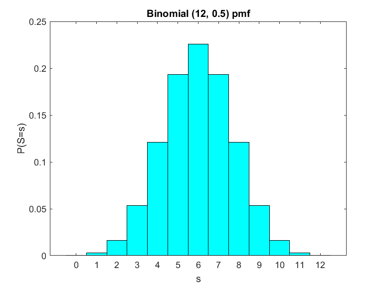
$ \text{Binomial(}12 ,0.5) \text{distribution} $
To see what it looks like, consider $ n=12 $ and $ p = \frac{1}{2}$. The pmf for the Bernoulli distibution is symmetric, with more of a chance of a number near the middle than at the 'tails' of the distribution. We refer to the outside edges of a distribution as the tails of a distribution. It makes sense that it is symmetric. For example with n=12, we know that $s=1$ is one success and $s=11$ is one fail. But the chance of a success or fail is the same, so the chances of a single success or a single fail over n attempts must the be same. Another way to say this is that we could simply rename fails as a success and vice versa, the distribution would then flip around its center on the x axis, but since $p$ does not change when it is one half (because now a success still has a probability of one half in each trial) then the distribution must remain the same. Hence it is symmetric.
Now consider what happens when we change $ p $.
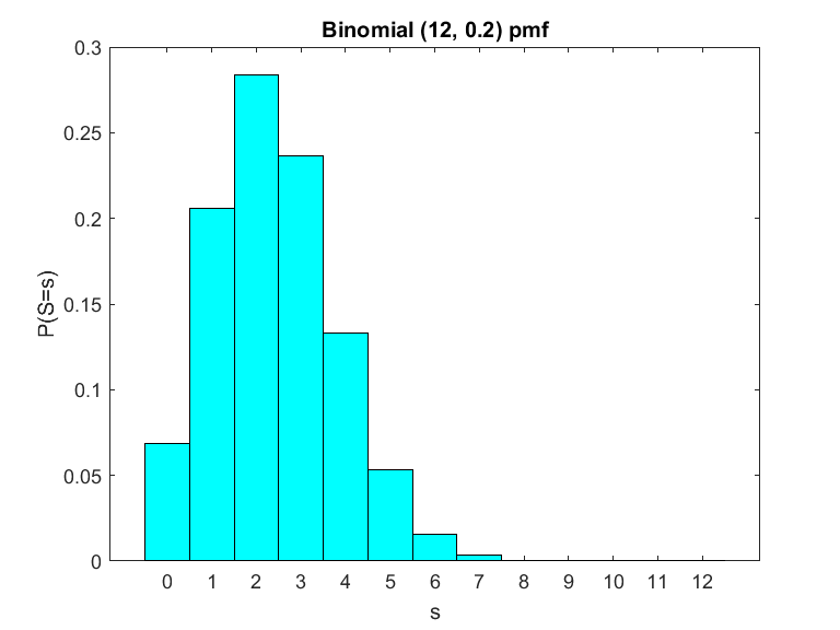
$ \text{Binomial(}12 ,0.2) \text{distribution} $
When the probability of a success is less than one half, the distribution is skewed to the right. This makes sense since now it is much less likely that we get a large number of success, and more likely that we get a large number of fails, since the chance of a success in any of the individual trial is small.
Regardless of $ p $, the distribution has a mean and a variance (as well as other moments). We can compute these using our formulas. But first we might start with some intuition. If for each of the trials we have a $ p $ chance of a success, it seems reasonable that over multiple trials the mean of the sum of successes is simply the number of successes times the mean of each success. This is true for this distribution (although not in general, for reasons we get into next chapter). That this is correct can be verified by applying our formula, although the calculation requires a trick. See the box for details. For now we will simply state the formulas for the mean and variance. They are $$ \text{E[S]} = n p $$ $$ \text{Var(S)} = n p (1- p) $$
To see how we can use this distribution to make useful calculations, we turn now to some examples
3.6 Continuous Random Variables and Distributions
The distributions we have seen so far are discrete distributions. However there are also continuous distributions, where the support or outcomes are not countably finite in number
The distributions we have seen so far are examples of discrete distributions. A discrete distribution is one where we can count the number of possible outcomes (values x can take). Often, we can think of examples where this is not true, the number of outcomes is infinite.
- The height or weight of a person
- rainfall measurements
- the time it takes to complete a task
- Incomes of a country
All of these can take on any value in some range, and between any two points in this range that could be outcomes there are an infinite number of other points that these random variables could take on (etc). This makes these variables CONTINUOUS random variables. You can rightly say that we can only measure to a certain accuracy, for example weights can only be measured to a certain accuracy, so we can make any of the above random variables into discrete variables by rounding. This is true but a) We are talking about reality, not measurement per se and in reality these are continuous b) It turns out that for many things we want to do working with continuous random variables is actually easier than working with discrete random variables, and in fact we will approximate a lot discrete distributions with continuous ones.
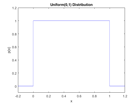
Since continuous distributions have an infinite number of outcomes, we do not use tables to describe the distribution. Instead we need to use formulas. Generically we will write these formulas as $p(x)$, they will be functions of the possible outcomes $x$ and are defined on some range for $x$. For example for the Uniform(0,1) distribution, the formula is $$ \text{p(}x) = \begin{cases} 1 & \quad \text{if }0 < x < 1\\ 0 & \quad \text{otherwise }\\ \end{cases} $$ We refer to $p(x)$ as the density of the random variable $X$ and the probabilities are called a probability density function (pdf). This is the continuous random variable analog of the pmf we saw for discrete random variables.
As always our probability distribution must satisfy the Kolmogorov axioms. So this function must always be nonnegative. Since we also require that probabilities sum to one, then the same must be true here. Her of course though we need to integrate. So it must be that for all probability distributions for continuous variables that $$ \int_{-\infty}^{\infty} \text{p}(x)dx = 1 $$ Note that by convention if the pdf is not defined for some ranges of $x$ then we set the pdf to zero, hence the integral above still makes sense.
For our Uniform(0,1) distribution this clearly makes sense. We have $$\begin{equation} \begin{split} \int_{-\infty}^{\infty} \text{p}(x)dx &= \int_{0}^{1} dx \\ &= [x]_{0}^{1} \\ &= 1-0 \\ &= 1 \end{split} \end{equation} $$ We could see this easily since the distribution is a box, so the area under the curve is simply base (1) times height (1) which equals one.
More generally probabilities for continuous distributions can be obtained by integrating under the probability density function. So we have that $$ P[a < X < b] = \int_{a}^{b} \text{p}(x)dx $$
As with discrete random variables, we can define the expected value of a function of $ X $ such as $ g(X) $. We replace the sum with an integral, but otherwise the expectation is as before. So we have $$ E[g(X)] = \int_{-\infty}^{\infty} g(x) \text{p}(x)dx $$. The mean and variance of $ X$ are special cases. The mean of a conintuous random variable, still denoted $\mu$, is defined with $ g(X)=X $ and is $$ \mu = E[X] = \int_{-\infty}^{\infty} x \text{p}(x)dx. $$ The variance, $ \sigma^2 $, defined with $ g(X) = (X - \mu )^2 $, is $$ \sigma^2 = E[(X - \mu)^2] = \int_{-\infty}^{\infty} (x - \mu)^2 \text{p}(x)dx $$
For the uniform distribution, we can see easily from the pdf that the mean is one half. Mathematically when we apply the formula we obtain $$\begin{equation} \begin{split} \mu &= \int_{-\infty}^{\infty} x \text{p}(x)dx \\ &= \int_{0}^{1} x dx \\ &= \frac{1}{2} [x^2]_{0}^{1} \\ &= \frac{1}{2} \end{split} \end{equation} $$ For the variance, we have $$\begin{equation} \begin{split} \sigma^2 &= \int_{-\infty}^{\infty} (x-\mu)^2 \text{p}(x)dx \\ &= \int_{0}^{1} (x-\frac{1}{2})^2 dx \\ &= \int_{0}^{1} (x^2+\frac{1}{4} - x) dx \\ &= [\frac{x^3}{3}]_{0}^{1} + \frac{1}{4} - \frac{1}{2} [x^2]_{0}^{1}) \\ &= \frac{1}{3} - \frac{1}{4} \\ &= \frac{1}{12} \end{split} \end{equation} $$ As with the sample variance, it is hard apart from relative sizes between variances of random variables to get the meaning of the value of the variance of a random variable. However it will turn out that the variance is important in understanding the basic issues presented in this course.
A worked example for a continuous random variable is available here.
3.7 The Normal Distribution
There are many continuous distributions, useful for different statistical problems. However one distribution is ubiquitous throughout statistics, so ubiquitous that it is called the normal distribution.
The normal distribution is the most commonly used distribution. We will see in Chapter 6 that it arises naturally in many statistical situations. It is this distribution that people often refer to as the bell curve (although there are other bell shaped distributions).
We can consider such a model for things like
- The height or weight of a person
- Rainfall measurements
- Incomes of a country
The curve has a number of intresting properties.
- It is symmetric around the mean
- It is more likely that an outcome is near the mean than far from it.
- There is very little chance of seeing outcomes quite far from the mean.
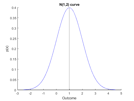
Like the binomial distribution, we can characterize this with a formula (even though in practice we will use computer or tables to actually work out probabilities). The formula is $$ p(x) = \frac{1}{\sqrt{2 \pi \sigma^2 }} \exp{ \left( -\frac{1}{2 \sigma^2} (x- \mu)^2 \right)} $$ You do not have to remember this formula, or work with it. We let computers do the work here, although for exams we have tables to solve problems.
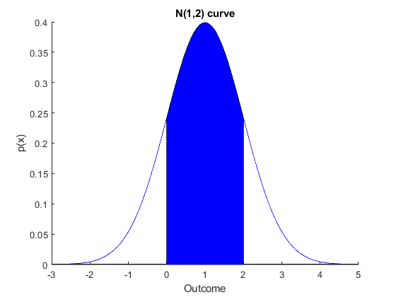
The nice thing about the normal curve is that the parameters of the curve are also the mean and variance. We have that $\mu$ is the mean, and $\sigma$ is the standard deviation. We will write a normal variable as $X \sim N(\mu, \sigma^2)$ and if the mean and variance are zero and one respectively we refer to the distribution as the standard normal distribution. So in the figure above the mean is one and the variance is 2. Often we use the random variable $Z$ for this.Most usefully for us, as we see in the later part of the course, is that we can compute probabilities of things we need by looking at the area under the curve. For any $a \le b$ we have $$ P[a \le X \le b] = \int_{a}^{b} \frac{1}{\sqrt{2 \pi\sigma^2 }} \exp{ -\left( \frac{1}{2 \sigma^2} (x- \mu)^2 \right)} dx $$ This is not nice to compute by hand, again we will use computers or tables to do this. But what we are computing can be seen in the figure below. Here the shaded area is $P[0 \le X \le 2]$ for a $N(1,2)$ random variable.
So how to do this? With tables (as you will use in the exam). See here for how to do this. Otherwise you need to use a computer, and the answer depends on the program. In excel you can compute $P[X \le x]$ using the command NORMDIST(x,mean,standard deviation,TRUE) where mean is the mean of your distribution and standard deviation is the standard deviation of your distribution (i.e. numbers). In matlab the command would be normcdf(x,mean,standard deviation).
More generally for a $N(\mu,\sigma^2)$ distribution, we need to first transform the distribution to one that has mean zero and variance one. For the discrete case we show below in the next section that if we add a constant to a random variable, it shifts the mean by that constant but does not change the variance. This makes intuitive sense, it is like picking up the distribution and placing it somewhere else, without changing the shape (so the shape is unchanged, hence the spread is unchanged).
So if the mean changes by what you add to it, and we have a random variable with mean $\mu$, then to change the random variable so that it has mean zero we could simply subtract the mean from the random variable. Mathematically we construct a new random variable $X-\mu$. This works for any random variable, so works also for the normal random variable. We have $$ E[X-\mu] = E[X] - \mu = \mu-\mu = 0. $$ So this transformation 'centers' our distribution on zero, we will indeed refer to this as centering.
How to fix the variance also comes from the results we will look at for the descrete case in Section 3.8. There we will see that multiplying a random variable by a constant changes the variance of the random variable by the square of whatever we multiply it by. What we want here is that the variance is equal to one, but have the variance equal to $\sigma^2$. So the transformation is to divide the random variable $X$ by the standard deviation $\sigma$. This also works for any random variable. We have that $$ Var \left( \frac{1}{\sigma}X \right) = \frac{1}{\sigma^2}Var(X) = \frac{1}{\sigma^2}\sigma^2 = 1. $$ We call this 'standardizing', and will refer in class to this with this word.
So putting this all together we have that the centered and standardized random variable $X$ is $$ Z = \frac{X-\mu}{\sigma} \sim N(0,1). $$ So now we can take any general normal, turn it into a standard normal, and we can use the tables. We will be doing a lot of this, so make sure you understand it. Not just for using the tables, it is a function we take in Chapter 8 all the time to understand hypothesis testing.
One thing you might be worried about here is that the probability calculations for the general normal and standard normal may not be the same. The following math might help here: $$\begin{equation} \begin{split} P(a \le X \le b) & = P(a-\mu \le X-\mu \le b-\mu) \\ & = P \left( \frac{a-\mu}{\sigma} \le \frac{X-\mu}{\sigma} \le \frac{b-\mu}{\sigma} \right) \\ & = P \left( \frac{a-\mu}{\sigma} \le Z \le \frac{b-\mu}{\sigma} \right). \end{split} \end{equation} $$ Since we are doing the same thing to both sides the probabilities stay the same.
3.8 Functions of a Random Variable
In practice we need to manipulate random variables, to construct estimators and tests later. Generating new random variables as functions of old ones is easy or hard depending on how complicated the initial random variable is and also how complicated the function is. We will start with both of these being very easy. Generically we refer to creating a new random variable $R=g(X)$.
For the general idea, consider the example where we have an $X$ random variable with the distribution
| $X$ | $P(X=x)$ |
|---|---|
| -1 | 0.3 |
| 0 | 0.4 |
| 1 | 0.3 |
Now consider the random variable that arises from $R=g(X)=2X$. To construct our new random variable we need to first work out what values $R$ takes. Since $X$ takes the values {-1,0,1} then $2X$ must take the values {-2,0,2}. Since $R=-2$ when $X=-1$ then it follows that $P[X=-1]=[R=-2]=0.3$. Following this logic we have that the new random variable has pmf
| $R$ | $P(R=r)$ |
|---|---|
| -2 | 0.3 |
| 0 | 0.4 |
| 2 | 0.3 |
Now consider a different function, where $R=g(X)=X^2$. Again, to construct our new random variable we consider what values $R$ takes. Since $X$ takes the values {-1,0,1} then $R$ takes the values {0,1}, since $0^2=0$ and $-1^2=1^2=1$. Since $R=1$ occurs when $X=-1$ or $X=1$, it follows that $P[R=1]=P[X=-1]+P[X=1]=0.3+0.3=0.6$. So we have the distribution
| $R$ | $P(R=r)$ |
|---|---|
| 0 | 0.4 |
| 1 | 0.6 |
This is basically an accounting exercise, one just needs to be careful. For continuous random variables this is a lot harder and one uses calculus methods to do this.
Since the function of a random variable R is still a random variable, then it has a mean and a variance and a distribution. All these can be calculated. When it comes to the mean or variance calculation, we basically have two ways of doing this. For functions $R=g(X)$, it will be true that $$ E[R] = \sum_{all r} r P[R=r] = E[g(X)] = \sum_{all x} x P[X=x] $$
For example, consider our example above where $Y=2X$. We have using the distribution for $R$ that $$ ER = \sum_{all r} r P[R=r] = -2*0.3+0*0.4+2*0.3 = 0 $$ or we could have calculated $$ Eg(X) = \sum_{all x} x P[X=x] = 2*(-1)*0.3 + 2*0*0.4 + 2*1*0.3 = 0.$$ It should be obvious that these are basically the same calculations.
.From this we can derive two quite useful results regarding some special (but ones we use a lot) functions of a random variable. It is always true that
- For $R=a+X$ that $ER = a +EX$ and $Var(R)=Var(X)$
- For $R=bX$ that $ER = bEX $ and $Var(R)=b^2 Var(X)$
The first of these should be intuitive, if I add a number to all the outcomes then all I do is shift the distribution by that number, so the balancing point of the distribution is shifted by that number. In terms of the variance, nothing happens to the spread of the distribution since it is merely shifted so the variance stays the same.
The second of these is somewhat intuitive. Multiplying $X$ by a number spreads it out, but also shifts the distribution (up if $b \ge 0$). So the mean shifts and the variance increases.
We can prove these results easily for discrete distributions (actually for continuous distributions the proofs are pretty easy too - try it). We have for the first claim for the mean $$\begin{equation} \begin{split} \mu_r &= E[X+a] \\ &= \sum_{all x} (a+x)P[X=x] \\ &= \sum_{all x} aP[X=x] +\sum_{all x} xP[X=x]\\ &= a \sum_{all x} P[X=x] + EX \\ &= a + EX \end{split} \end{equation} $$ which is $ER$ as claimed.
For the second claim, we have for $R=bX$ that $$\begin{equation} \begin{split} \mu_r &= E[bX] \\ &= \sum_{all x} (bx)P[X=x] \\ &= b \sum_{all x} x P[X=x] \\ &= bEX \end{split} \end{equation} $$ Thus the claim is shown.
For the variance here we have $$\begin{equation} \begin{split} Var(bX) &= E[bX-E(bX)]^2 \\ &= E[b(X-EX)]^2 \\ &= \sum_{all x} (b (x-\mu_x))^2 P[X=x] \\ &= b^2 \sum_{all x} (x-\mu_x)^2 P[X=x] \\ &= b^2 Var(X) \end{split} \end{equation} $$ and so that result is true also.
This might all look like meaningless math, but it has its uses. In particular it shows how we are able to transform a $N(\mu, \sigma^2)$ random variable into a $N(0,1)$ random variable, which is a calculation we will make a lot of use of.
Copyright © Graham Elliott
Distributed By Themewagon