
8. Hypothesis Testing
It will often be the case that theories give strong implications for measurements we make. In these cases we want to consider the question of whether or not the theory is correct or not having taken the relevant measurements. In this situation we would like to make a decision rule, basically we would like to have a set of procedures for which once we observe data that we use a statistical method to say either the theory is wrong or alternatively that we cannot say that the theory is wrong given the data. Suppose our theory suggested that the mean should be zero, and we observe data that we are sure is representative. Our sampling results suggest that our measurements can be thought of as a draw from a distribution with mean zero. But we have seen, through the randomness that arises from taking observations, that the sample mean will not be equal to zero even if the theory is correct. So we need some rule that says that the sample mean is too far away from zero to reasonably be considered that the data is being drawn from a distribution with mean zero. Intuitively, we then expect that the rule will be based on this distance, which we will see is true.
"By a small sample, we may judge of the whole piece." - Miguel de Cervantes, from his novel, Don Quixote.
8.1 The Classical Approach
For hypothesis testing to be relevant, you must have a theory that you are trying to test. Recall our discussion in the introduction about how science is typically done --- we observe the world then try and come up with rationalisations about why we see what we see. The theory predicts how the world operates. To formalize this for a particular problem, we need the theory to predict actual means for some random variable which describes data we can observe. In the speed of light example our theory might suggest a particular value for the speed of light and our measurements of this speed are the outcomes of the random variable we can actually observe. Economists and other scientists typically derive mathematical models for the phenomenon they are trying to describe complete with parameters that must take certain values or ranges of values for their theory to hold. We then need to relate these parameters to means of distributions for the data, so that we can think about what our hypothesis says the mean of the distribution for each observation should be.
This can be stated more formally. As in the last chapter, consider each observation we are going to observe $x_{i}$ as an outcome from the random variable $X_{i}$. Our theory has suggested a value for the mean $ E[X_{i}]$ of the distribution of $X_{i}$ that accords with our theory and also a range of values for this mean that does not accord with our theory. All of the hypothesis tests we examine will have this feature. It is part of the hard work of science to boil down stories about the world to direct implications about the random variables that describe the data we are able to measure. But once done, as we are about to see, we can then ask the question of whether or not our data supports our theory or not.
For each problem we will want to be able to determine the a value for the mean which accords with our theory, which we write as $$ H_0 : \mu = \mu_0 $$ where $\mu_0 $ is the value for which the mean is what our theory predicts it should be. This is called the null hypothesis. The capital H stands for hypothesis and the subscript zero indicates that it is the null hypothesis.
Values for which our theory is considered incorrect are collected together and named the alternate hypothesis (as in the alternative to the null). There are typically two possibilities for what values for μ would indicate that our hypothesis is not true. The first is when our theory would be incorrect for values for the mean either greater than the null value only or smaller than the null value only. When the theory is incorrect for values greater than the null value the alternative hypothesis is $$ H_a : \mu > \mu_0 $$ When the theory is incorrect for values smaller than the null hypothesis value the alternative hypothesis is $$ H_a : \mu < \mu_0 $$ In either of these situations we refer to the alternative as being a one sided hypothesis for the reason that we are only going to conclude against the theory if the sample mean is too far to one predetermined side of the null value. In the first case, where we will consider the theory untrue if it appears that a more reasonable value for μ is larger than the null hypothesis value, we call the test an upper tail test (the reason for this name will become clear in the development of the testing methods below). For the second case we refer to the testing situation as a lower tail test.
The second possibility is that we would disbelieve our theory if both seeing a sample mean that is too large or too small would invalidate our hypothesis. Here the alternative hypothesis is given by $$ H_a : \mu \neq \mu_0 $$ This is known as a two sided hypothesis for reasons that should be clear.
Some examples will make things more concrete.
Example 1 - Normal Example This example has to do with quality control. A manufacturer has a cereal box filler machine that is supposed to put 16 ounces of cereal in each box. The manufacturer knows the machine is not perfect and that the actual distribution of the filled boxes is normal with a standard deviation of .4 The producer takes a random sample of 25 boxes and finds that the boxes have an average weight of 16.2 ounces. The question the manufacturer may want to ask is, if the machine is overfilling and should be adjusted. Now the null hypothesis for the producer would be that the machines are working fine, i.e. $ \mu_0 = 16$ , and that the average weight of 16.2 ounces is just through random variation. The alternative hypothesis might be either a two sided alternative (they lose profits if they overfill, might get fined if they underfill) or a one sided alternative (lax enforecement means no fines, so they do not care if it is underfilling a bit) where $ \mu>16 $ is the alternative.
Example 2 - A Large Sample Example We can consider a test of the efficient markets hypothesis, which says that average returns (in the absence of risk) are zero. The hypothesis says nothing about the size of the variance, but I will assume that individual returns are normal, i.e. $ X \sim N(0,\sigma^2). $ Our sample of 61 observations might result in $ \bar{x}=0.2 $, and we might have an estimate of the sample variance of $X$ at $\sigma^2=0.05$. Our null hypothesis is that $ \mu_0, $ so the sample mean of 0.02 is just from sampling error. Our alternative here would be two sided --- being able to make consistent losses is just as good as being able to make consistent profits, but you want to do the opposite of what the trader says!
Example 3 - Proportions This is based on a CNN poll on cloning. The question asked if respondents approved of human cloning for medical research purposes. The sample size was 507 and the response rates were
| Choice | Sample Proportion |
|---|---|
| Approve | 0.54 |
| Disapprove/No idea | 0.46 |
We would be interested in the possibility that less than (or equal to) 50% of the people in the country approve.
we asked if support was less than or greater than 50%. One way to set this up is $$\begin{equation} \begin{split} & H_0 : p = 0.5 \\ & H_a : p > 0.5 \end{split} \end{equation} $$ The reason for choosing it this way is that we are really wondering if the estimated 54% support is just randomly above 50% or not. We could also have set this up as $$\begin{equation} \begin{split} & H_0 : p < 0.5 \\ & H_a : p > 0.5 \end{split} \end{equation} $$ As we will see, it is much easier to do hypothesis testing if the null has an "equal" sign instead of an inequality. Here the answers would end up the same. If it is unlikely that a mean of .5 generates an estimate of 54%, then it is LESS likely that a smaller mean does. So choosing the largest in the range of possible means makes sense.
The classical testing procedure seeks to make a decision rule; i.e. tell us when we either accept or reject the null hypothesis. That is, we want to know if
- is true, so the null is accepted; or
- is true, so the null is rejected.
We often say that "not rejected" instead of "accepted." This is a somewhat semantic difference based on the Popperian view of scientific method where all models (i.e., null hypotheses) are considered only provisionally true. The best analog is found in the law: is a defendant "not guilty" or "innocent?". Usually an acquittal is an admission that there is not sufficient evidence to be sure of guilt, rather than a decision that the person is truly innocent.
Unfortunately, even though this all seems clear cut, in practice it is not. Recall my cards example where I draw cards from a deck with replacement. Even if the cards were 50-50 red and black, there is a chance that I would many reds and no blacks (it is possible). This means that the method always involves errors. It is easiest to see when I draw a table;
| Choose Null | Choose Alternative | |
|---|---|---|
| $ H_0 $ is true | correct | Type 1 error |
| $ H_0 $ is true | Type II error | correct |
Thus we have a classification system for the errors: Type I Error: We reject when is true; i.e. we wrongly conclude our model was wrong. Type II Error: We fail to reject when the alterative is true; i.e. we wrongly conclude that the model is correct.
As we will see in the next section, it is usually impossible to remove both errors, and more annoyingly reducing one increases the other. We will need to choose a tradeoff between them that we are comfortable with.
8.2 The Hypothesis Testing Procedure Heuristically
We will start with formalizing the intuition, and then complete the formalization in a step by step procedure in the following section. Consider a problem where we have a one sided (upper tail) hypothesis testing problem. We write the null and alternative as $$\begin{equation} \begin{split} & H_0 : \mu = 0 \\ & H_a : \mu > 0. \end{split} \end{equation} $$ In this case our null hypothesis says that the true (or maintained) mean is equal to $\mu_0=0$. Assuming our null hypothesis to be true then $\bar{X}$ is distributed normally with mean $\mu_0 $ and variance $ \sigma^2/\sqrt{n}. $ I will set $ \sigma^2/\sqrt{n} =1 $ for this example.
So, a $\bar{x}$ that is large relative to the mean $\mu_0$ will suggest that the null is not true and that the alternative is mored likely. Further, because we know the sampling distribution of $\bar{X}$, we know what types of $\bar{x}$ to expect. But how large should $\bar{x}$ be before we decide that the mean is not really $\mu_0?$. Suppose we choose a value $k>0$, and decide that all observed sample means above this cutoff will be classified as rejecting the null hypothesis and all those below $k$ will be classified as not rejecting the null hypothesis.
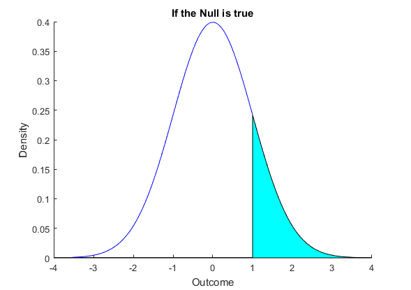
The Type 1 error from choosing $k$ as a cutoff , meaning the error we would make if we chose this rule, is the probability that $\bar{X}>k$ when the mean really is zero. This is shown in Figure 1 below where I have chosen $k=1$. If we choose this value as a cutoff, we can easily work out the probability that we reject even though the null hypothesis is true. This value, which we call Type I error, is $$\begin{equation} \begin{split} P[\bar{X}>k] &= P \left[ \frac{\bar{X}-\mu_0}{\sigma/\sqrt{n}} > \frac{k-\mu_0}{\sigma/\sqrt{n}} \right] \\ &= P \left[ Z > 1 \right] \\ &=0.1587 \end{split} \end{equation} $$ This is the shaded area in Figure 1. We might think this chance of an error too large, we can easily make it smaller by making $k$ larger. This is to say that we would choose a larger cutoff before we decide that our null hypothesis is not correct.
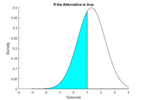
Increasing $k$ does reduce Type I error, however it makes Type II error larger as well. Consider Figure 2. Here we have the same cutoff $k$ as in Figure 1, i.e. we set $k=1$. But in this case we are assuming that the alternative is true, that $\mu$ is not zero but 1.3. Now what happens? We defined Type II error as the probability that we do not reject when the alternative is true. This is the $P[\bar{X}<1]$. This is pictured in Figure 2, where the relevant area is shaded. We can also compute this probability. $$\begin{equation} \begin{split} P[\bar{X}<k] &= P \left[ \frac{\bar{X}-\mu_0}{\sigma/\sqrt{n}} < \frac{k-\mu_0}{\sigma/\sqrt{n}} \right] \\ &= P \left[ Z < (1-1.3) \right] \\ &=0.3821 \end{split} \end{equation} $$
We can see from the Figures that we can increase $k$ to reduce Type I error, but it comes directly at the expense of increasing Type II error. From the Figure consider increasing $k$, any movement to the right must make the area under the curve less than this value in Figure 2 bigger as it is decreasing the area under the curve in Figure 1. This means that we have a tradeoff to deal with - we need to trade off Type I error with Type II error.
The classical approach chooses Type I error to be fairly small, say in the range of 0.01 to 0.1, although in an extreme amount of cases in real research 0.05 is chosen (to see where this comes from, see Box XX). In this case we can work out the level for %k% we need to choose for any particular Type I error choice. Consider our centering and scaling transformation. We have $$\begin{equation} \begin{split} P[\bar{X}>k] &= P \left[ \frac{\bar{X}-\mu_0}{\sigma/\sqrt{n}} > \frac{k-\mu_0}{\sigma/\sqrt{n}} \right] \\ &= P \left[ Z > \frac{k-\mu_0}{\sigma/\sqrt{n}} \right] \end{split} \end{equation} $$ We want this equal to 0.05, so we use the tables to find the $k$ or more generally $\frac{k-\mu_0}{\sigma/\sqrt{n}}$ that would work. For Type I error equal to 0.05, this is $\frac{k-\mu_0}{\sigma/\sqrt{n}}=1.645. $
Again using the results of the previous chapters, we can easily compute probabilities such as $P[\bar{X}>k]$ for any value k by simply transforming the problem to a standardized normal, i.e. $$\begin{equation} \begin{split} P[\bar{X}>k] &= P \left[ \frac{\bar{X}-\mu_0}{\sigma/\sqrt{n}} > \frac{k-\mu_0}{\sigma/\sqrt{n}} \right] \\ &= P \left[ Z > \frac{k-\mu_0}{\sigma/\sqrt{n}} \right] \end{split} \end{equation} $$ Some more terminology. We usually refer to Type I error as the size of the test. The value for $\frac{k-\mu_0}{\sigma/\sqrt{n}} $, i.e. the cutoff after we have centered and standatdized, is called the critical value of the test. Different sizes will lead to different critical values. Finally, all this was undertaken for a test that rejects only for large values. For one sided tests where we reject for small values, we simply reverse everything above.
The second possibility is that we would disbelieve our theory if both seeing a sample mean that is too large or too small would invalidate our hypothesis. Here the alternative hypothesis is given by $$ H_a : \mu \neq \mu_0 $$ This is known as a two sided hypothesis for reasons that should be clear. In this situation we would need a cutoff for when the sample mean was too large, denote this as $k_u$ for the upper cutoff, and one for where the sample mean is too small denoted $k_l$.
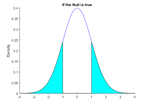
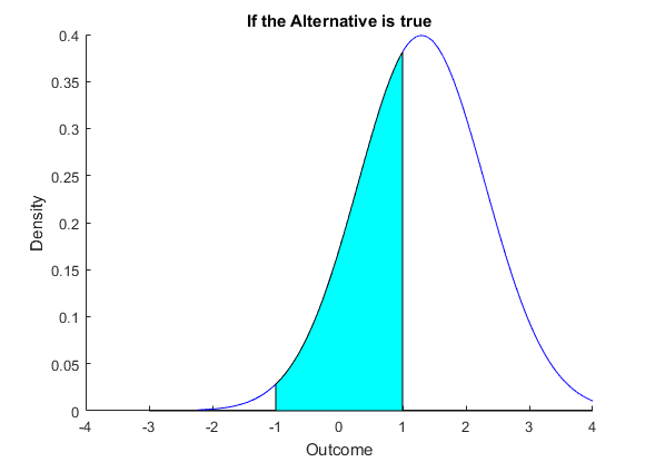
We again consider an example where the null hypothesis is that the mean is zero. As in the one-sided example we set $ \sigma^2/\sqrt{n} = 1$ Figure 3 gives the distribution when we assume that the null is true and use an upper and lower cutoff equal to plus and minus one. Figure 4 again considers the situation that our alternative is true and that the true mean is 1.3, leaving the variance the same. In both Figures we have shaded the areas for which we make a decision error. When we are assuming that the null hypothesis is true, Type I error (or size) is the sum of the areas outside the cutoffs. These are the sample means for which we would incorrectly decide that the null hypothesis was not true. In Figure 2 the wrong decision is when we choose the null hypothesis even though the alternative is true. So the Type II error in Figure 4 is the area between the cuttoffs.
Again, as in the one sided situation, we make both Type I and Type II errors. The wider we spread the cutoffs around the null hypothesis mean, the smaller is the Type I error. However looking at Figure 4 this clearly would increase Type II error. Hence we again have a tradeoff between the errors. The fix is as in the one sided case, we choose a small but nonzero size (which is Type I error). Notice that here though because the Type I error is the sum of the probabilities in each tail, to construct the critical values for any size we need to have half the size in one tail of the distribution and the other half in the other tail (there is no need to be half-half so long as they add up, but since the distribution is symmetric then spreading size evenly makes some sense). So to construct a test of size 0.05 we realise that we want to solve for $$\begin{equation} \begin{split} P[\bar{X}>k_u] &= P \left[ \frac{\bar{X}-\mu_0}{\sigma/\sqrt{n}} > \frac{k_u-\mu_0}{\sigma/\sqrt{n}} \right] \\ &= P \left[ Z > \frac{k_u-\mu_0}{\sigma/\sqrt{n}} \right] \\ &=0.025. \end{split} \end{equation} $$ From the tables this is setting $\frac{k_u-\mu_0}{\sigma/\sqrt{n}}=1.96$
Finally, we should realize that since the normal distribution does not reach zero in the tails, there is no cutoff so that we can be completely sure that Type I error is zero (that we never falsely reject the null). Even though this is true, note that we can be so close to a probability equal to one that most people would find it convincing, although see Box XX.
8.3 A Step by Step Approach to Testing Hypotheses
Having seen how hypothesis tests are constructed somewhat heuristically, we take a more constructive approach. Note that we need to justify somehow the distribution we use for our test.
We will use a four step procedure for construcing tests. The steps are
- Determine the null and alternative hypotheses.
- Choose size and compute critical values.
- Construct the t statistic.
- Decide whether or not to reject the null hypothesis.
Step 1 - the null and alternative hypotheses We have covered this earlier. It is important to understand the problem you are trying to resolve with the test. Successfully testing a hypotheses measn that we can determine which parameter values fit our theory and which parameeter values lead to invalidation of our theory. For the purposes of this course, where we concentrate on theories regarding the mean, this results in just knowing if a large value, samll value (which each result in one sided tests) or both (which results in a two sided test) leads to our theory being incorrect.
Step 2 - Choosing size and constructing the critical values Choosing a reasonable size for a test should be more controversial than it is in practice, even amongst science in the top journals of each field typical choices are in the 0.01 to 0.1 range, with 0.05 being the most popular. Once size is chosen (or given to you) then we need to compute critical values. This involves understanding the distribution of the test statistic we compute in the next step. For the purposes of this course however it is always the normal distribution, either because $X_i$ are all normally distributed or because we have applied the central limit theorem and we are using the normal distribution as an approximation. It is always important for interpreting your result to know if you have an exact normal distribution or you are using an approximation. For this reason we will always be clear on this. Either way though we compute critical values based on the normal distribution, so our critical value calculations always take one of the three following forms. Let $\alpha $ be the size of the distribution. Then we have the following three possibilities.
| Test type | Calculation | For $\alpha = 0.05 $ |
|---|---|---|
| Upper 1 tail test | $P[Z>z_{\alpha}]=\alpha$ | $ z_{\alpha}=1.645 $ |
| Lower 1 tail test | $P[Z<-z_{\alpha}]=\alpha$ | $ z_{\alpha}=1.645$ |
| Two Sided test | $P[Z<-z_{\alpha/2}]+P[Z>z_{\alpha/2}]=\alpha$ | $ z_{\alpha/2}=1.96$ |
The results for other values for $\alpha$ can be determined from the normal tables or computer
Step 3: Construct the test statistic Up to now we have always centered and standardized our estimate, then compared to the normal distribution. Since we are always doing this, it is easier just to define the statistic we want as the centered and standardized estimate as the object we are interested in. This is generally knows as the t statistic (sometiems Z-score), and is defined as $$ t = \frac{\bar{x} - \mu_0}{\sqrt{\sigma^2/n}} $$
Step 4: Decide whether to reject or not We compare the t statistic, which is where on the normal curve we have our draw from the data, with our critical values we determine in step 2. In the previous section where we discussed intuitively the testing problem, we noted that we rejected for a one sided test if the sample mean was too large or too small relative to the cutoff. Since the numerator of the t statistic is just the distande between the sample mean and null value for $\mu_0$, we do the same thing for the t statistic. For a upper one tail test we reject the null hypothesis if the t statistic is too large (above the critical value for an upper tail test) or too low (below the critical value for a lower tail test). If we are doing a two tail test we have both upper and lower tail critical values and reject if the t statistic is either too large or too small.
To see the method in action, we return to our three examples for the chapter.
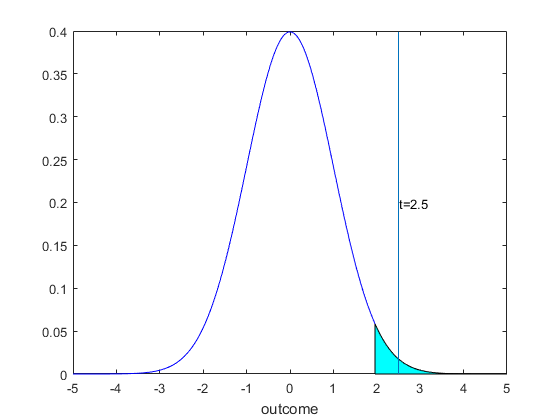
Example 1 For this example, we have already determined the null and alternative hypotheses in Step 1, to repeat we determined that $$\begin{equation} \begin{split} & H_0 : \mu = 16 \\ & H_a : \mu > 16 \end{split} \end{equation} $$ For Step 2, we realize that because the $X_i$ are normally distributed with unknown mean but variance equal to $0.4^2$, that the sample mean is exactly distributed as a normal distribution with variance $0.4^2/25$. Hence there is no need to approximate the distribution, we know the distribution is normal and so we can use this distribution to get an exact critical value. Choosing size to be $0.05$, and realizing that this is an upper tail test, we determine that the critical value $z_{0.05}=1.96 $. For Step 3, we compute the t statistic. We have that $$\begin{equation} \begin{split} t &= \frac{\bar{x}-\mu_0}{\sigma/\sqrt{n}} \\ &= \frac{16.2-16}{0.04/\sqrt{25}} \\ &=2.5. \end{split} \end{equation} $$ Our t statistic here is very large, far from zero. For Step 4 we realize that this is above the critical value of 1.96, so we reject. We can see this in the following figure.
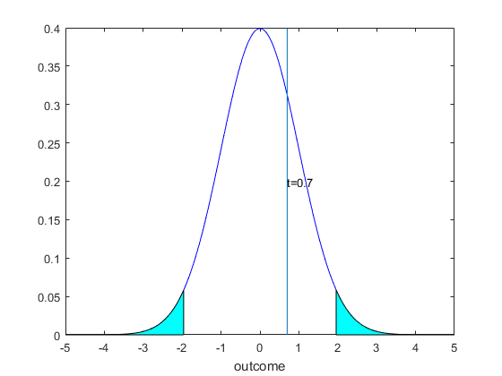
Example 2 Again we have already determined Step 1 earlier, we have that our null and alternative hypotheses for this example were $$\begin{equation} \begin{split} & H_0 : \mu = 0 \\ & H_a : \mu \neq 0 \end{split} \end{equation} $$ So for this problem we have a two sided test, we reject for large and small values. For Step 2, we need to determine the size and critical value. Choosing size to be 0.05, we will split this into an upper part of 0.025 and a lower part of the same value. For our distribution, since we do not know that returns are normally distributed, and we had to estimate the variance, we do not have that the sample mean random variable is exactly normally distributed. However, we can appeal to the central limit theorem and approximate our distribution with a normal distribution. Recall for this we need to justify that the approximation is reasonable. In this case we do not expect returns to be very skewed, however we might think that returns are not independent. However, suppose we are satisfied with the approximation, this means that the upper and lower critical values are 1.96 and -1.96.
For Step 3, we compute the t statistic. We have $$\begin{equation} \begin{split} t &= \frac{\bar{x}-\mu_0}{s/\sqrt{n}} \\ &= \frac{0.2-0}{0.05^2/\sqrt{61}} \\ &=0.7. \end{split} \end{equation} $$. For Step 4, we compare to the critical values. The t statistic value of 0.7 is well inside our region where we do not reject the null hypothesis. So we conclude that the trader does not have special abilities to generate profits and the efficient markets hypothesis holds here. We can visualize this in Figure 6.
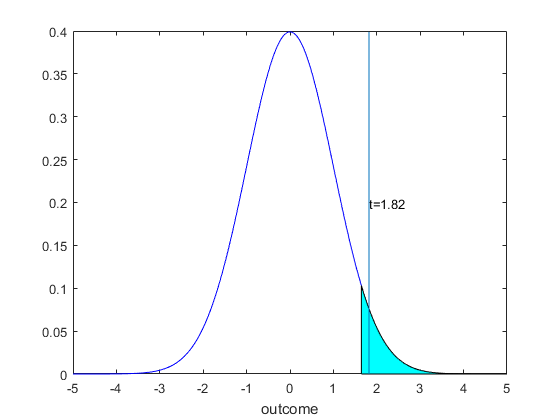
Example 3 For the poll example, we again have already undertaken step 1. We decided earlier that the null and alternative hypotheses were $$\begin{equation} \begin{split} & H_0 : p = 0.5 \\ & H_a : p > 0.5 \end{split} \end{equation} $$ For Step 2, choose size equal to 0.025. Since we have a one tailed upper tail test we work the critical value out to be equal to 1.96. This is the size of the area shaded in Figure 7. In terms of the distribution, we again have a normal distribution as an approximation via the central limit theorem. Recall that we could have used the Binomial, but since the sample size is large this is not a good approach. And because under the null hypothesis the distribution of each datapoint is symmetric, we expect that with a sample size this big the normal approximation will be very good.
For Step 3, we determine the t statistic. We have $$\begin{equation} \begin{split} t &= \frac{\bar{x}-p_0}{\sqrt{\frac{p (1-p)}{n}}} \\ &= \frac{0.54-0.5}{\sqrt{0.5(1-0.5)/25}} \\ &=1.82. \end{split} \end{equation} $$ For Step 4 we notice that this is in the rejection area (greater than the critical value) so we rejection the notion that there is a 50-50 split (and accept the alternative that a majority of the population is in favor). Visually we see this in Figure 8.
Notice that we could have used an alternative estimator of the standard deviation, i.e. we could have used the sample mean $\bar(x) $ rather than the null hypothesis value $p_0$ to construct the t statistic. We would have had in the denominator $ \sqrt{0.54(1-0.54)/507}=0.022 $ instead of what we used above, i.e. $ \sqrt{0.5(1-0.5)/507}=0.022 $. Clearly there is no difference for this problem, since our value for the sample mean is close to the null mean. In practice this rarely changes the result of the test, and if it does it means that the t statistic must be close to the bounds both ways. which we might not find too persuasive in terms of the choice between rejecting and failing to reject the hypothesis.
8.4 The p-value Approach
The method we have seen so far in the last section is a standard approach to testing. However there is a dual approach that leads to exactly the same rejection regions. This dual approach is called the p-value approach, and is often popular because it lets the reader choose the size of the test rather than having this imposed by the researcher. From time to time however the p-value approach has been controversial, see Box XX
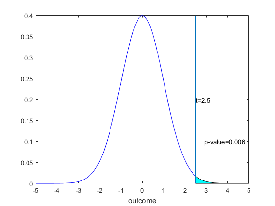
Consider the first example (cereal boxes) and recall our picture of the testing approach and decision. Repeating Figure 5:
For our one sided upper tail test, we rejected our null hypothesis because the t statistic of 2.5 was above our critical value of 1.96. We recall that this critical value was chosen because the shaded area in Figure 5 was equal to 0.025 in probability, or more formally $P[Z>1.96]=0.025$. Consider what this means for a t statistic. We already understand that if $t<1.96$ we fail to reject and if $t>1.96$ we reject. We could have said this a different way. If it is indeed the case that $t>1.96$, this is the same thing as saying that the $P[Z>t]<0.025$. This must be so because if the shaded area is 0.025 then the area under the curve for any number greater than 1.96 must be smaller. Similarly, we can only have $t<1.96$ if the $P[Z>t]>0.025$. This is because now the t statistic would have to be to the left of 1.96, so the area in the tail of the normal distribution would be larger than size. This suggests that we could simply report $P[Z>t]$ and compare this to size to decide whether or not we reject or fail to reject. Clearly the answer would have to be the same as the approach in Section 8.4, so the two approaches are in this sense dual's of each other.
The reporting of $P[Z>t]$ (for a one sided upper tail test) is known as the p-value approach, where the p-value is simply the $P[Z>t]$. Reporting this value is sufficient for any size test - we simply reject if the p-value is less than the size we want to choose and fail to reject if it is larger than the size we want to choose. As noted in the previous paragraph, using the p-value in this way leads to precisely the same answer as the approach in Section 8.3.
For full hypothesis testing, the approach refined to a steps is as follows.
- Determine the null and alternative hypotheses.
- Choose size
- Construct the t statistic and determine the p-value
- Reject if the p-value is smaller than size, otherwise fail to reject.
The steps are basically the same, which is of course not surprising. The difference is that no critical values need to be computed. Instead we compute the p-value (which as a task has exactly the same difficulty). The result is the same at the end in terms of each sample being either rejected or failing to reject either way.
Above we described the construction of the p-value for the one sided upper tail test. It was to work out the $P[Z>t]$. In a picture (for the example 1 t statistic of 2.5) this is simply
This is the type of calculation we have been doing since Chapter 6
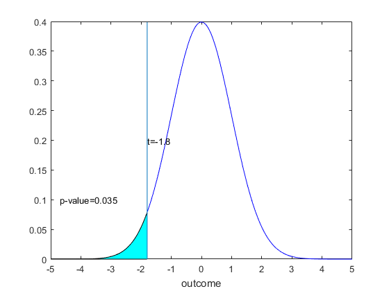
For the one sided lower tail test, we take the mirror image. In this case we want to construct the probability that we could have seen a more extreme sample (further from the null) than we did, we would compute the p-value to be the $P[Z< t]. $ Here I chose a t statistic of -1.8, so the p-value is 0.035. Clearly at a size of 0.05 we do not reject (the critical value for this would have been -1.645) but we do reject for a size of 0.025 (where the critical value would have been -1.96). The p-vlaue allows us to quickly choose for any size given.
For a two sided test, things become a little more complicated because we have to consider both sides of the distribution. However the complication is small. The best way to think about it is to think of the p-value as the probability of getting a more 'extreme' sample than the one we actually saw. In the one sided upper tail test this is the probability of a larger t than the one we saw, for a one sided lower tail test this is the probability of a smaller t than the one we saw. For a two tail test, a more extreme sample would be in both directions, i.e the probability of seeing a t statistic greater than $|t|$ plus the probability of seeing a t statistic smaller than $-|t|$. We can picture this in the following Figure, where the p-value is now the sum of the areas in the tails, i.e. the shaded area under the curves.
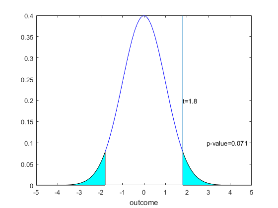
In this case then we want to compute, using the symmetry of the normal curve, $2P[Z>|t|]$ as the p-value. Thus we really just need to remember to multiply by 2. That we need to consider both sides comes back to being able to compare the p-value to the size of the test in order to come to the same decision. Since for a size $\alpha$ two sided test we choose our upper and lower areas to be equal to $\alpha/2$, we need to either compare $P[Z>|t|]$ to $\alpha/2$ or instead double the probability and compare to $\alpha$. Both work, we choose the latter approach so that in every case we are comparing the p-value to size.
We can summarize this in a table.
| Test type | p-value Calculation |
|---|---|
| Upper 1 tail test | $P[Z>t]$ |
| Lower 1 tail test | $P[Z<t]$ |
| Two Sided test | $2P[Z> |t|]$ |
You might have seen that there is some controversy over the use of p-values in research, including some journals that have banned them. For more discussion on this look here.
8.5 The Power of a Test
We have completely defined the hypothesis testing, and seen two eqivalent methods for arriving at a decision as to whether or not the null hypothesis is correct or not, without any consideration of the size of type II error. The notion of power is a look at the extent of Type II error and the issues around it for interpresting statistical results.
The power of a test is informative about the ability of a test to actually distinguish between the null and alternative hypotheses. Imagine a test of a new drug, which in truth actually is better than the drugs being currently used for the condition they are all designed to treat. It is possible that the new drug actually does not look so good in a clinical trial just by chance, i.e. in the trial the sample mean measuring the outcome we obtain is small relative to the true mean. However, this can be due just to the sampling error we have been examining in Chapter 6, even with a well run clinical trial. We can approximate the sampling distribution, for example suppose we have the sampling distribution depicted in the following figure. Here the true mean is $55\%$, but it is reasonable to see samples of where $\bar{x}$ is $50\%$ or less. Now suppose that current drugs have a cure rate of $50\%$. Then it would seem quite likely that we obtain a sample estimate from the clinical trial that suggests the new drug is worse than existing drugs because the estimate is not precise enough to really distinguish between means of $50\%$ and $55\%$. Computations of power are intended to shed light on when this situation occurs versus situations where the test might have a good chance at distinguishing between the means.
Recalling that we do not know what $\mu$ actually is equal to (if we did we would not be out finding data to estimate or do tests on it), all of our calculations for the hypothesis tests are a 'what if' analysis, more directly 'what if the null is true and the mean is $\mu_0$. We compute the t statistic as though this is true, and assuming it is true we have $$ t = \frac{\bar{X} - \mu_0}{\sigma /\sqrt{n}} \sim N(0,1). $$
Now consider a different 'what if' scenario. Suppose that this is a one sided test that rejects for large values. Choose $\mu_1$ to be a value from the alternative region, so $\mu_1 > \mu_0$. If $\mu_1$ is the true value, this means that the t statistic under the null is not centered on the correct value. We want to fix that, which we do with the following algebra. We have $$\begin{equation} \begin{split} t &= \frac{\bar{X} - \mu_0}{\sigma/\sqrt{n}} \\ &= \frac{\bar{X} - \mu_1 + \mu_1 - \mu_0}{\sigma/ \sqrt{n}} \\ &= \frac{\bar{X} - \mu_1}{\sigma/\sqrt{n}} + \frac{\mu_1 - \mu_0}{\sigma/\sqrt{n}} \\ &= \frac{\bar{X} - \mu_1}{\sigma/\sqrt{n}} + k \end{split} \end{equation} $$ Now the first term is correctly centered when $\mu_1$ is the true mean and the second term is just a number, set it equal to $k$ as in the equation. So the distribution of the t statistic under the 'what if' scenario that the alternative is true and $\mu_1$ is the correct mean is a normal distribution. When we add the second part to the normal distribution the mean is now $k$.
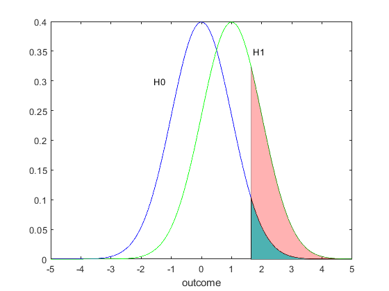
We can draw the distribution (Figure 11) under the null hypothesis (which assumes the mean is $\mu_0$) and also under the alternative hypothesis (which assumes the mean is $\mu_0$). For the test we reject the null hypothesis (wrongly, this is Type I error) equal to the area under the curve above the critical value with a probability equal to the size of the test. This is the green shaded area. On the same figure we can draw the distribution under the alternative hypothesis (which assumes the mean is $\mu_1$). We can compute under this distribution the probability that the t statistic is larger than the critical value, i.e. $P[t>z_{\alpha}]$. On the figure this is shown as the sum of the green and pink areas. This is a larger number, and tells us the probability that the test chooses the correct outcome, that the null hypothesis is not true. This area is the power at $k=1.$
Consider testing the hypothesis $$\begin{equation} \begin{split} & H_0 : p = 0.5 \\ & H_a : p > 0.5 \end{split} \end{equation} $$ The following two figures, analogous to Figures 1 and 2 on page 2, present the sampling distribution of $\bar{X}$ under the null hypothesis (that the mean is $50\%$) and also under the assumption that the mean is $55\%$, which is a choice of a value in the alternative hypothesis. However instead of computing Type II error, we compute the power which is one minus Type II error.
One hard part of understanding power is understanding how to compute it. In Figure XX above, we are computing the probability that a test of the null that the mean is $0.5$ rejects if the true mean is actually $0.55$. So the test is set up as though the null is true, but probabilities are calculated as though one of the values in the alternative is true (in this example 0.55). Here is the calculation. The test rejects if $$ t = \frac{\bar{x}-0.5}{\sqrt{0.5*(1-0.5)/n}} $$ is greater than the critical value {z_{\alpha}} (for this one tailed test). What we want to calculate then is the probability this happens when the true mean is not $0.5$ but is instead $0.55$. This means that we need to recenter on the correct mean. In math we have $$\begin{equation} \begin{split} P[t>z_{\alpha}] &= P \left[ \frac{\bar{x}-0.5}{\sqrt{0.5*(1-0.5)/n}} >z_{\alpha} \right] \\ &= P \left[ \bar{x} >0.5+z_{\alpha}\sqrt{0.5*(1-0.5)/n} \right] \\ &= P \left[ \frac{\bar{x}-0.55}{\sqrt{0.55*(1-0.55)/n}} > \frac{-0.05+z_{\alpha}\sqrt{0.5*(1-0.5)/n}}{\sqrt{0.55*(1-0.55)/n}} \right] \\ &= P \left[ Z > \frac{-0.05+z_{\alpha}\sqrt{0.5*(1-0.5)/n}}{\sqrt{0.55*(1-0.55)/n}} \right] \end{split} \end{equation} $$ It is worth going through the steps of this equation. The first step is the usual probability that the t statistic exceeds the critical value, which would be $\alpha$ if the mean we are assuming for the calculation was $0.5$. However since we are assuming the mean is $0.55$, the sample mean is not correctly centered. The next line simply rewrites the statement inside the probability to be a statement about the uncentered sample mean, i.e. we simply undo the centering and standardizing. Now that we have isolated teh sample mean on the left hand side ofthe inequality, we cetner and standardize using the correct value for $p$ (and by correct value I mean the one we are assuming is the true one for the calculation). Once we have centered and standardized with the mean set to $0.55$, we have that the centered and standardized sample mean has either an exact $Z$ distribution or an approximate $Z$ distriubution and we can make the calculation. Choosing size to be 5%, we have for a sample size of $n=$, that this probability is ...
The next part of understanding this is to consider what these numbers mean. If the null were true, we would reject the null with size %\alpha%, in this example $5\%$. But if the alternative we picked were true, the chance we reject jumps up only to $X\%$, which is not much higher. Thus there is a very big chance that even if the null were false, we still would not be able to reject the null. In this sense we say that the test has very little power of distinguishing the hypotheses, because if either the null or alternative is true the chances of rejecting or not rejecting do not change. Suppose instead we found that power was one, i.e. that the probability of rejecting jumps up to one under the chosen alternative. This would mean that we can often distinguish the hypootheses. Indeed, power equal to one means we never make a Type II error, so the only times we make an error is the $5\%$ of times we erroniously reject the null when it is true. So high power means a large chance of distinguishing the hypotheses.
The approach we took to computing power in the above example is the correct way to approach the problem in general. The first step is to choose one of the many possible values for the mean from the alternative. We could have chosen any value for $p$ above 0.5. We could have undertaken the power calculation for all possible values above $0.5$, and constructed a power curve as a function of the alternative. This is commonly done. However in terms of understanding a particular study, it is usually more informative to choose a single value under the alternative as we did above and do the calculation for that value. The value of the mean you would choose is one for which you hope the test actually has high enough power that you trust that you can interpret a failure to reject as evidence for the null hypotheses, rather than simply something we expect under either the null or alternative hypothesis (which is how we interpret lower power tests).
8.6 Issues and Intuition with Testing Hypotheses
Now that we have learned how to construct and interpret tests, it makes sense to step back a little and think of the big picture when it comes to hypotheses testing
Hypothesis Testing clearly is at issue with Step 3 of the scientific method discussed at the start of this course. Once we have a theory, we find implications of the theory and test these implications. The implicatinos then become the null hypotheses, and after writing this down as a random variable any parameters that do not fit the implications become the alternative hypothesis.
In many instances when we work with data, there is no obvious theory to test. Some fields are deeply in the first step of the scientific method, attempting to measure things without having formed strong theories to explain the data they have. (Psychology?). Other fields are more deeply developed, and are more closely attuned to tesing theories (LHC and physics?).
Figures here
One aspect of hypothesis testing that should always be considered in working with them is that hypothesis tests are a statistical method, when we talk about say rejecting the mean to be zero we often say that the mean is statistically significantly different from zero (or significant, in shorthand). When we say statistically signficant, we mean only what we say, that we can statistically distinguish possible means. But this does not mean that the difference between the measn we can distinguish are scientifically meaningful. For example in
Whilst in some situations a hypothesis test might not be the obvious approach to answering a question, in all statistical work we do want to understand how precise any estimate we report is. In the next chapter we see that dealing with the precision of an estimator is intinitely linked with hypothesis testing.
Copyright © Graham Elliott
Distributed By Themewagon