
Worked Example for Bivariate Random Variables - Discrete RVs
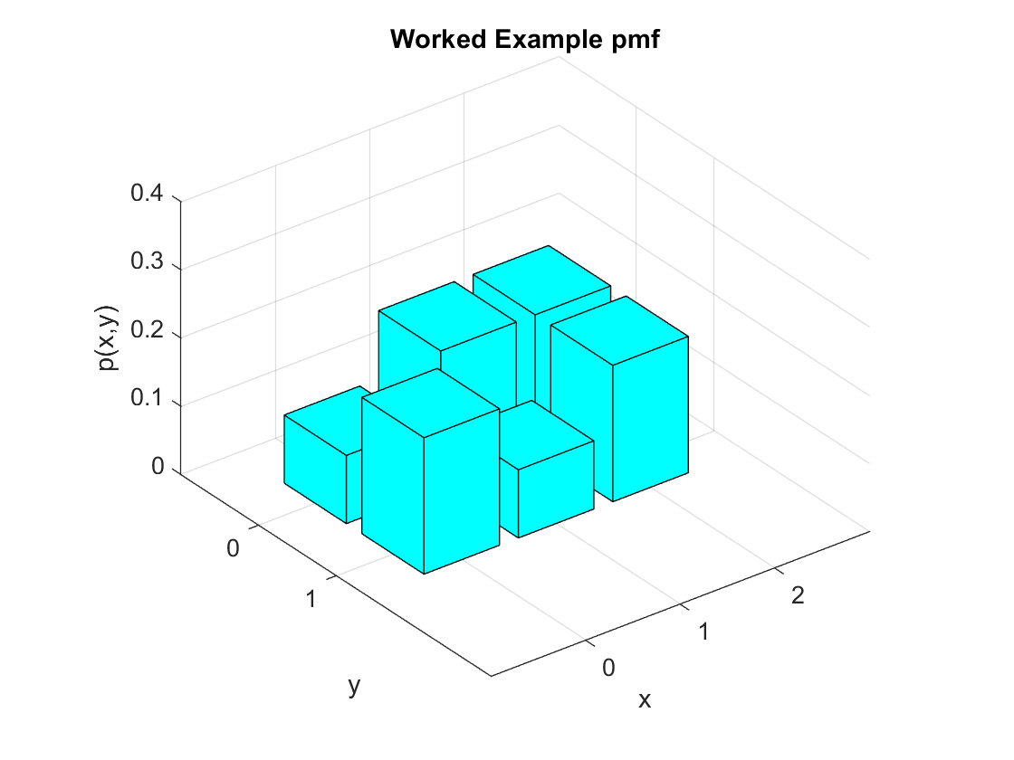
This page works through all the ideas of Chapter 4 for a discrete bivariate random variable. Our $X,Y$ random variables have a probability distribution as in the following table.
| X\Y | 0 | 1 |
|---|---|---|
| 0 | $ 0.1 $ | $ 0.2 $ |
| 1 | $ 0.2 $ | $ 0.1 $ |
| 2 | $ 0.2 $ | $ 0.2 $ |
So here our $X$ variable takes on one of three possible values, $X=0,1,2$ and our $Y$ variable takes on either zero or one. The probabilities in the table are our joint distribution of $X$ and $Y$. For example $P(Y=0,X=1)=0.2$.
We can determine the marginal distributions from the joint distribution. Recall that our general formula for the marginal distribution for $Y$ is $$ P[Y=y] = \sum_{all \: x} P[X=x,Y=y]. $$ This is just summing down the columns, for the marginal distribution for $X$ we sum out the $Y$ dimension which is summing across the rows. So the joint distribution with the marginal distribution is given by
| X\Y | 0 | 1 | P[X=x]= |
|---|---|---|---|
| 0 | $ 0.1 $ | $ 0.2 $ | $ 0.3 $ |
| 1 | $ 0.2 $ | $ 0.1 $ | $ 0.3 $ |
| 2 | $ 0.2 $ | $ 0.2 $ | $ 0.4 $ |
| P[Y=y]= | $ 0.5 $ | $ 0.5 $ | sum = 1 |
Now that we have the marginal distributions we can easily work out things like the mean of $X$ or $Y$. For the mean of $X$ we have $$ EX = \sum_{all \: x} xP[X=x] = 0x0.3 + 1x0.3 + 2x0.4 = 1.1. $$ For the mean of $Y$ we can easily see it is $0.5$ without working it out carefully (but feel free to check using the formula).
We can also work out conditional distributions for either $X$ or $Y$. Recall that the general formula for $Y$ given $X$ is $$ P[Y=y|X=x] = \frac{P[X=x,Y=y]}{P[X=x]}. $$ Consider calculating the conditional distribution of $Y$ given that $X=2.$ We have that $$ P[Y=y|X=2] = \frac{P[X=2,Y=y]}{P[X=2]} = \frac{P[X=2,Y=y]}{0.4}. $$ At $Y=0$ we have $ P[Y=0|X=2] = 0.2/0.4 = 0.5 $ and $ P[Y=1|X=2] = 0.2/0.4 = 0.5. $ So the conditional distribution here is a one half chance of either a zero or one.
Because the conditional distribution is indeed a distribution, it has a mean and variance. We see immediately that the conditional distribution here for $Y|X=2$ is a Bernoulli distribution with a probability of success $p=0.5$ (same as a coin flip). So immediately we know the conditional mean $E[Y|X=2] = 0.5$ and the conditional variance $Var(Y|X=2) = 0.5.(1-0.5) = 0.25 $.
You probabily noticed that the conditional distribution for $Y|X=2$ is the same as the unconditional or marginal distribution for $Y$ (bottom line of the table). We also recall that we have independence when the conditional distributions are equal to the marginal distribution. But $Y$ and $X$ are not independent - the euqivalence of the conditional distribution and marginal distribution meaning independence requires this equivalence for all conditional distributions (so for all values for $x$.) We can see that they are not independent by checking the equivalence for any of the other values for $X$. For example $P[Y=1|X=0] = 2/3$, which does not equal the marginal distribution for $Y=1$ which is $0.5$. Finding a single discrepency tells us that the random variables are not independent.
We can also work out the covariance, but this is not a neat result here. Recall that the covariance is given by $$ \sigma_{XY}=E(X-\mu_X)(Y-\mu_Y)P[X=x,Y=y] $$. For this example we have already worked out that $\mu_X = EX = 1.1 $ and $\mu_Y = 0.5 $. So all that remains is plugging the numbers in and doing the calculation.
We have $$\begin{equation} \begin{split} E(X-\mu_X)(Y-\mu_Y) &= \sum_{\text{all x}} \sum_{\text{all y}}(x-\mu_X)(y-\mu_Y)P[X=x,Y=y] \\ &= (0-1.1)(0-1/2) 0.1 +(0-1.1)(1-1/2)0.2+(1-1.1)(0-1/2)0.2+(1-1.1)(1-1/2)0.1 \\ &+ (2-1.1)(0-1/2) 0.2 + (2-1.1)(1-1/2) 0.2 \\ &= -\frac{6}{100}. \end{split} \end{equation} $$
So there is a negative correlation. To examine the strength of the correlation we would need to work out not just the covariance but also the correlation.
Copyright © Graham Elliott
Distributed By Themewagon