9. Confidence Intervals

Typically in casual conversation we tend to refer to estimates --- say the mean or a correlation --- as though it were the true value for some larger population instead of an estimate of this underlying parameter from a sample. When you are writing a technical report, or a news story, it kills the flow a bit to have to give qualifications when you are trying to give an idea of some 'average' value. For example its sounds nicer to say that "60% of the population believe that the president is doing a poor job" rather than "somewhere near 60% of the population believe that the president is doing a poor job". The first sounds better but the problem is that we have no idea from the reporting of a sample mean as to how precise an idea of the true value the estimate gives us.

It is a fundamental idea of this course that it is not correct to consider an estimate as the truth. So when the polling agencies report that 60% of the population believe that the president is doing a poor job we know that the proportion is not exactly six out of every ten people, but some value close to this proportion. When a scientist reports that there are 100 billion stars in the milky way, this too is an estimate. But knowing how good an idea the estimate gives us of the truth is important in understanding what the value '60%' or '100 billion' really means.

Hence the first challenge we have (which will be solved this chapter) is to find a way of reporting our estimate and also reporting some indication of how close we expect it to be to the value of the feature of the problem we are trying to estimate. In the last chapter we solved this challenge through the use of hypothesis tests. When we had an idea of what the parameter to be estimated was --- namely the null hypothesis $\mu_0$ --- we could examine how reasonable it was that the data we had resulted from a sample with a true mean of $\mu_0$.But what happens when we do not have a particular theory or value for $\mu$ in mind? How can we even compute our sample distribution for $\bar{X}$ since it is centered on the true mean, which we are estimating precisely because we do not know it? This is the second challenge, how to compute the probabilities of various samples without knowing the true centering value. This is the second challenge, which will also be solved in this chapter. The notion of confidence intervals kills both these birds with its single stone.

9.1 The Uncertainty in the Estimate

Simply conveying the estimate has the problem that it does not in any way convey any indication of how certain we are that this is a good estimate. We may know that the truth is 'close' to this number, but we do not know how close. For example, suppose the above polling proportion of $60\%$ arose from asking $5$ people, of which three believed the president was doing a poor job. In this case we know that the true sample proportion could easily be $50\%$, since even if $p=\frac{1}{2}$ we still have $XX\%$ chance of seeing a sample mean of $60\%$ or more. However we are far more certain as to the true proportion if it were a poll of a thousand people where 600 believed the president was doing a poor job. In this case if the true $p=\frac{1}{2}$ then the chance of seeing a sample mean of $60\%$ or more is $XX\%$. We have the math to understand this, in chapter XX we saw that the sample mean has a sampling distribution and that it is not eactly the true mean of the distribution. We further saw that the precision of the estimate was related to the standard error of the estimate, which in turn was smaller the larger the number of observations. This follows directly from our result that the distribution gets tighter and tighter around the true value as the sample size increases. We can use this evaluation of the sampling distribution to making statements about the uncertainty over what the mean might be for any observed sample. The idea will be to think about all the possible true means that might have led to a sample like the one we observed.

First, to illustrate why understanding the uncertainty is important, consider the following two examples.

For each of these examples, we have presented the problem of uncertainty over the true mean in terms of whether or not the data is able to resolve arguments between different theories that may have been proposed for the generation of the data. In both cases the different theories come down to different views about what the true mean is, but it is possible (more so in the poll example) that various possible means could have generated the data. A reasonable way then of reporting the uncertainty over the sample average then might the to collect all of the possible values for the true mean into a set of values, and report this as the set of possible means suggested by the data. When this set is very large, then we would regard the data as not being very precise about where the true mean is and hence uncertainty is large. Alternatively, a very small set of values for the mean that are compatible with the data would then suggest that we have a precise estimate. Precision then is directly how many or few values for the mean are compatible with the data.

There is a problem, however. Suppose that the true mean is $\mu$. Then we know that the sample distribution, supposing the conditions behind the central limit theorem apply, will be $N(\mu,\sigma^2/n)$). We have seen that the normal distribution has tails that never actually get to zero, hence it is possible even though the mean is $\mu$ that we get any possible $\bar{x}$. How could we rule out any possible $\mu$ since any $\mu$ is compatible at some probability with the sample mean we computed? The answer is going to be similar to that of the last chapter when we hit this problem --- we are going to be willing to ignore any $\mu$ for which the sample generated has a very low probability of being seen.

9.2 Inverting Tests to obtain Confidence Intervals.

We now turn to a constructive way of obtaining a set of models, here a set of possible means, for which the data could have been generated from. Because any model could have generated the data, we will again use our notions of probability to compute a set that is as small as possible given a probability statement. We need to be careful in interpretation however, remembering that the model is fixed and that the data is a random draw from its distribution.

The basic idea will be to describe the uncertainty over the true mean through reporting all of the possible null hypotheses that cannot be rejected using the hypothesis test methods of the previous chapter.

The problem of not knowing $\mu_0$ is then solved by taking each one in turn, pretending it is true, and then seeing if it is likely to be compatible with having generated the sample with high enough probability. In this sense this chapter does not involve learning new methods of statistics, just that we report the results from the hypothesis testing in a different way because we are asking a slightly different question. The question of the last chapter was 'Does my data fit my model?', and of this chapter is 'what models fit my data?'.

Just as in the last section we need to choose a size for all of the hypothesis tests. This is typically the same size over all tests, so lets call this again $\alpha$. Recall that $\alpha$ is the probability that when the chosen null hypothesis however we observe a sample that leads us to reject this hypothesis. Rather than report this number $\alpha$, we typically report the number $1-\alpha$ which is the called the coverage rate of the confidence interval. The reason for the name and the use of $1-\alpha$ instead of $\alpha$ will be clear after we explain the method.

We define a confidence interval with coverage rate of $1-\alpha$ as the set of null hypothesis values that cannot be rejected using a test of size $\alpha.$

Typically we would use a two tailed test, although the definition does not require this however confidence intervals based on two sided tests have been found to be the most practically useful. Given this definition, it is not surprising that the way we are going to calculate the confidence interval turns out to be almost identical to how we computed hypothesis tests. The only difference is that we do it many times so that we can work out which of the null hypotheses are rejected and which ones are not. But we will see an easier way mathematically.

Consider our standard testing problem for some chosen $\mu_0$. Assuming this mean is the true mean, we will fail to reject null hypotheses of the form $$\begin{equation} \begin{split} & H_0 : \mu = \mu_0 \\ & H_a : \mu \neq \mu_0. \end{split} \end{equation} $$ if $$ -z_{\alpha/2}< t( \mu_0 )< z_{\alpha/2} $$ where $$ t(\mu_0) = \frac{\bar{x}-\mu_0}{se(\bar{x})} $$ Here I have through the notation $t(\mu_0)$ made the dependence of $t$ on the chosen mean explicity. The reason for this is that we are going to hold the sample fixed, so hold $\bar{x}$ and its standard error $se(\bar{x})$ constant, and vary $\mu_0$. As we increase $\mu_0$ we see that $t(\mu_0)$ is a declining (linear) function. We can represent this on the following Figure using the values from Example 1 from last chapter.

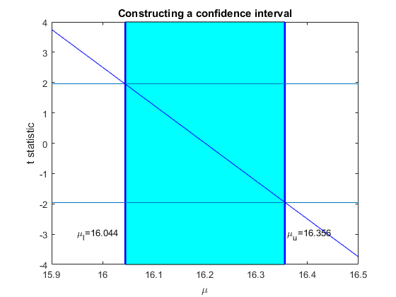
The downward sloping line is $t(\mu_0)$ where we have possible values $\mu_0$ on the x axis and the t statistic on the y axis. As $\mu_0$ moves away from $\bar{x}=16.2$ in either direction, then $t(\mu_0)$ gets further away from zero. Eventually there will be values for $\mu_0$ that result in the value of $t(\mu_0)$ exceeding the critical value in each direction (depicted here as $\pm 1.96$). All of the values for which the sloping line is in between the critical values are values for the null hypothesis that fail to reject. If we collect these values for which we fail to reject, this is the confidence interval. We depict this by the vertical lines where the downward sloping line crosses the critical values for the t statistic. The values for $\mu$ between the vertical lines is the confidence interval.

In practice we do not have to look at all the possible values for the null hypothesis here. Looking at the picture we see that the lower bound occurs precisely when our t statistic hits the upper critical value, and the lower bound happens precisely when we hit the lower critical value. All of the points of the confidence interval are inside these two bounds, so we can directly compute the bounds. First consider the lower bound for $\mu$ which occurs when the t statistic hits the upper critical value. Recall that for Example 1 in the last chapter $\bar(x)=16.2$, $\sigma=0.4$ and $n=25$. So we want to solve for $\mu$ such that $t(\mu_l)=1.96$ (we are constructing a confidence interval with coverage equal to $95\%$. So we solve in general $$ \frac{\bar{x}-\mu_l}{se(\bar{x})} = 1.96 $$ which solves to $$ \mu_l = \bar{x}-1.96se(\bar{x}).$$ For this example $$\begin{equation} \begin{split} \mu_l &=\bar{x}-1.96se(\bar{x}) \\ &= 16.2 - 1.96*\frac{0.4}{\sqrt{25}} \\ &=16.04 \end{split} \end{equation} $$ as in the Figure.

For the upper bound we again look at the Figure and see that the upper bound corresponds to the situation where $\mu$ is such that the t statistic is equal to the lower critical value. So we want to solve in general $$ \frac{\bar{x}-\mu_u}{se(\bar{x})} = -1.96 $$ which solves to $$ \mu_u = \bar{x}+1.96se(\bar{x}).$$ In terms of our example this is $$\begin{equation} \begin{split} \mu_l &=\bar{x}+1.96se(\bar{x}) \\ &= 16.2 + 1.96*\frac{0.4}{\sqrt{25}} \\ &=16.36 \end{split} \end{equation} $$ as in the Figure.

Finally, put all this together. Recall that the use of $\pm 1.96$ arose because we have a two sided test with size $5\%$ and yeilding a confidence interval with coverage $95\%$ More generally a $(1-\alpha)\%$ coverage requires use of critical values $\pm z_{\alpha/2}$ and the confidence interval bounds are $$ (\mu_l,\mu_u) = \bar{x} \pm z_{\alpha} se(\bar{x}). $$ This will be the formula we use to construct the confidence intervals in practice when $\bar{x}$ can be considered to have either an exact normal distribution or alternatively if we can apply the central limit theorem.

9.3 Understanding Confidence Intervals

In the last section we learned how to construct confidence intervals. We now turn to understanding their interpretation - precisely what do these upper and lower bounds represent. It is here that many researchers have difficulties, because the intuitive answer that they represent the 'most likely values with $95\%$ probability' is not correct.

Confidence intervals are intended to go a step beyond simply reporting the point estimate and allowing us to use the sampling error to consider what the data is telling us about reasonable values for $\mu$. To think about how the coverage rate should be understood, we first need to recall that $\bar{x} $ is a random draw from the distribution $\bar{X}$. This means that our confidence interval $$ \bar{x} \pm z_{\alpha} se(\bar{x}) $$ should be considered a random draw from many possible confidence intervals we might have seen where each is a draw from the distribution $$ \bar{X} \pm z_{\alpha} se(\bar{x}). $$

Consider any single draw which yields a single lower and upper bound for the confidence interval. The actual unknown but true value for $\mu$ is either inside the confidence interval or it is not inside the confidence interval. When we want to consider a probability statement on the interval, it will be the probability that the interval contains the true mean where we think of the probability as the frequency of times such an interval will contain the true (non random) mean of the distribution, the object we are trying to measure. So what we want to construct is the $$ P \left[ \bar{X}-z_{\alpha/2}se(\bar{X})<\mu< \bar{X}+z_{\alpha/2}se(\bar{X}) \right] $$ which if evaluated such that $\mu$ is the mean of $\bar{X}$ will give the probability that intervals constructed this way will contain hte true mean in the sense where the probability is the proportion of intervals that include $\mu$. We can rearrange this so that it is based on a centered and standardized statistic. We have $$\begin{equation} \begin{split} P \left[ \bar{X}-z_{\alpha/2}se(\bar{X})<\mu< \bar{X}+z_{\alpha/2}se(\bar{X}) \right] &=P \left[ -z_{\alpha/2}se(\bar{X})<\mu-\bar{X}< z_{\alpha/2}se(\bar{X}) \right] \\ &=P \left[ -z_{\alpha/2}se(\bar{X})<\bar{X}-\mu< z_{\alpha/2}se(\bar{X}) \right] \\ &=P \left[ -z_{\alpha/2}<\frac{\bar{X}-\mu}{se(\bar{X})}< z_{\alpha/2} \right] \\ &=P \left[ -z_{\alpha/2}<Z< z_{\alpha/2} \right] \\ &=1-\alpha. \end{split} \end{equation} $$

Although each of the steps is fairly easy it is worth going through them slowly. In the first step (right hand side) I subtracted off $\bar{X}$ from everything. For the second step I multiplied each term by $-1$ which flips the inequalities, so I also reversed the terms to keep the inequalities in the usual order. In the third step we divide by the standard error of the estimate, which is never negative so keeps the inequalities the same. In the fourth step I realize that the center object is the centered and standardized sample mean random variable, which either has an exact normal distribution (as I have written it) or an approximate one if we can use the central limit theorem. Finally, we can use our knowledge of the normal distribution to owrk out the probability. It is exactly (or approximately, if we use the clt) the coverage rate from the previous section.

We are now in a position to fully interpret the confidence interval. The coverage rate of $1-\alpha$ means that there is a $(1-\alpha)\%$ chance that a confidence interval will include the true $\mu$. It does not mean that $\mu$ has a $(1-\alpha) \%$ chance of being in the interval, because it is the interval that is random and not the $\mu$ we are trying to measure.

We also see from the probability calculation that constructing the interval as the set of null hypothesis values that cannot be rejected using a test of size $\alpha.$ generates an interval with exactly $1-\alpha$ coverage.

Clearly, we would like our confidence interval to be as short as possible. This would give is the most precise understanding of what reasonable values for the mean of $X_i$ might be. So what makes a confidence interval short or long? Mechanically we see that the length is decided by $z_{\alpha} se(\bar{x})$, since this is what we add and subtract in each case from the estimated sample mean. So either a smaller $z_{\alpha}$ or a smaller $se(\bar{x})$ will give us a shorter confidence interval.

A smaller $z_{\alpha}$ is only possible if we choose $\alpha$ to be larger, which means that the coverage of the confidence interval would have to be lower. This makes sense, if we simply choose to make the confidence interval shorter it will on average cover the true mean less often. Hence this is not usually an avenue to obtaining more precision!

The standard error of the esitmator (or equivalently the variance of $\bar{X})$ can be made smaller either through reducing the variance of $X_i$ or alternatively having a larger sample size. Often reducing the variance of $X_i$ is out of our control. In some cases we can control this, i.e. better measuring of what we are trying to measure can improve precision here. What is more often (although not in observational studes typically) under our control is the sample size. OFten in studies we could ensure that confidence intervals are short enough to be useful by working out how big a sample size we require for the confidence interval to be precise enough to distinguish interesting possible values for the mean from those that are not interesting.

9.4 Confidence Intervals and Polls

For polls, or more generally problems where the data are drawn from Bernoulli($p$) random variables, there are a few interesting issues that arise. For that reason we examine them separately.

We introduced confidence intervals as being collections of null values from a two sided test that cannot be rejected when the test has size $\alpha$. Then we saw that we could write the interval as $$ \bar{x} \pm z_{\alpha} se(\bar{x}). $$ Consider our third example from the last chapter (our poll). In this example we had $\bar{x}=0.54$ and $n=507$. We can compute our standard error of the estimate as $$\begin{equation} \begin{split} se(\bar{x}) &= \sqrt{\frac{\bar{x}(1-\bar{x})}{n}} \\ &= \sqrt{\frac{0.54(1-0.54)}{507}} \\ &= 0.0221 \end{split} \end{equation} $$ Our confidence interval is then $ 0.54 \pm 1.96*0.0221 $ which equals $(0.497,0.583)$. This is perfectly valid, and will be the way we construct the intervals in most cases.

However when we set up the testing problem for sums of Bernoulli random variables, that because the variance of a Bernoulli($p$) random variable is $p (1-p) $ that we could have used the null value for $p$ instead of our sample mean as we just did above. We could do this for a confidence interval, but clearly this makes for a difficult estimator. We would actually have to do the tests over and over again or come up with a new formula that takes into account that the t statistic is not exactly linear in the null value. In practice what we do is what we did above, that is we always choose to use the sample estimate in constructing our estimate of the standard error.

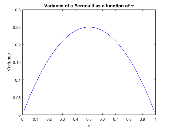
The second issue that arises is that, unlike the cases we have examined with a general sample mean in the earlier sections, is that we know for sure that $0 \le p \le 1.$ This has a few consequences. First, consider the standard error again and our knowledge of the bounds for the mean. A direct implication is that the variance of $X_i$ has an upper and lower bound. We can see this in the following figure, where we plot the variance $p (1-p)$ against $p$. Notice that it attains a maximum of $\frac{1}{4} $ at $p=\frac{1}{2} $.

Now look at the formula for the confidence interval. We have that the confidence interval is wider if we set the variance to be larger. But we could always choose the variance to be equal to the worst case, i.e. set $\sqrt{p (1-p)}=0.25$ which would make the interval wider. But the probability that the interval catches the true proportion will be larger than $1-\alpha$, but perhaps we are not worried by this. It would still be at least this level of coverage. If we do this our interval for a poll is now $$\begin{equation} \begin{split} CI &= \bar{x} \pm z_{\alpha} \sqrt{\frac{\bar{x}(1-\bar{x})}{n}} \\ & \approx \bar{x} \pm z_{\alpha} \sqrt{\frac{\frac{1}{4}}{n}} \\ &= \bar{x} \pm \frac{z_{\alpha}}{2} \sqrt{\frac{1}{n}} \end{split} \end{equation} $$ Bearing in mind that we typically choose a $95\%$ confidence interval, so $z_\alpha = 1.96 $, then we are essentially adding and subtracting $\sqrt{\frac{1}{n}}$. This makes constructing intervals for polls easy enough to do in your head, because you simply add and subtract the inverse of the square root of the sample size. For example, many polls have $n=1000$ or close to it. We can calculate that $\frac{1.96}{2} \sqrt{\frac{1}{1000}} = 0.031 $ or we could have simply used $\sqrt{\frac{1}{1000}}=0.032 $. Either way we simply add and subtract $0.03$ to get our confidence interval.

It is often the case when polls are reported that something called the 'Margin of Error' or MoE is reported. It is often this simple calculation, but in general refers to $1.96 \sqrt{\frac{\bar{x}(1-\bar{x})}{n}}$. For typical sample sizes of $1000$ or more used in polls each of the methods presented above will give you the same answer to two decimal places regardless of which you use unless the estimated probability is close to zero or one. But reporting this for you obviously makes life easy, you simply compute the confidence interval as the estimate plus or minus the MoE.