5. Sampling

We are finally in a position to consider the first main question we have been working towards throughout this course. The question we will answer in this chapter is "If our model is described by the random variable $X$, then what should the data look like if we obtain multiple observations?". We refer to this as sampling. We refer to a set of data (or random variables that describe the data) as a sample (hence our use of sample mean etc. in Chapter 2). Recall that our data sample with $n$ observations is $(x_1, x_2,....,x_n)$ We will think of these observations as draws from a set of random variables $(X_1,X_2,...,X_n)$, i.e. we have a random variable $X_1$ from which we see one draw (observation) $x_1$, and so on for the $n$ random variables and observations. The joint distribution of our data is the joint distribution of all $n$ random variables, and we consider our sample to be a draw from this joint distribution. Example: A doctor gives a drug to 100 patients, so we have 100 random variables $(X_1, X_2,...,X_{100})$ describing the outcome for each of the patients. Each patient observation (say cure or not cure, so these are all Bernouilli random variables) comes from its corresponding random variable. Typically, as in the previous chapter, we will not be intersted in the entire distribution. In this course, we are typically interested in the mean of the observations (i.e. the sample mean we examined in Chapter 2). Recall that the sample mean is $$ \frac{1}{n} \sum_{i=1}^{n} x_i. $$ We can consider having been drawn from a random variable $$ \frac{1}{n} \sum_{i=1}^{n} X_i. $$ So we are interested in a function of the random variables. In our drug example this would be the average cure rate.

5.1 Random Samples

Working with joint distributions of large numbers of random variables such as $(X_1,X_2,...,X_n)$ can be very tedious. Fortunately however there are assumptions that we can make that are both realistic for many real world situations where we collect data and also make the problem of understanding functions of the random variables somewhat straightforward and not too difficult. First, when each of the random variables are independent, we have through the independence rule we saw in the last chapter that the joint distribution simplifies greatly. For $(X_1,X_2,...,X_n)$ mutually independent of each other, we have that $$ P[X_1=x_1,X_2=x_2,....,X_n=x_n] = P[X_1=x_1]P(X_2=x_2]...P[X_n=x_n] $$ and so the joint distribution is the product of the marginal distributions for each random variable. So independence will be helpful.

A second simplification that arises naturally is that when we are taking multiple observations on the same thing (for example giving the same drug to a lot of patients and measureing their outcome) then it makes sense that all of the marginal distributions are equal to each other. This is to say that in many studies each observation is a draw from a distribution that is identical to the distributions that generate the other observations. This means of course that each of the random variables $X_i$ have the same mean and variance for all $i=1,...,n$

When both these assumptions hold, we call the sample a Random Sample. So the definition is that a random sample is a sample where the $n$ observations are drawn from $n$ independent random varaiables each with the same distribution.

We will use shorthand to describe this. For example suppose that the observations come from random samples all with the same $N(\mu,\sigma^2)$ distribution, we would write this as $X_i \sim iid N(\mu, \sigma^2). $ The 'iid' part stands for 'independent and identically distributed' although the 'identifically distributed' part is a bit redundant since they are all normal with the same mean and variance.

5.2 The moments of the sample mean

We will refer to the function $$ \bar{X} = \frac{1}{n} \sum_{i=1}^{n} X_i. $$ as the random variable that describes the sample mean. The distribution of this random variable is the 'Sampling distribution of the same mean'. We are going to be interested in the distribution of this function of the original random variables, however we will start with looking at the mean and variance.

For all of the calculations, assume that we have a random sample, so the data are independent and identically distributed.

First consider the mean. We have that $$\begin{equation} \begin{split} E[\bar{X}] &= E \left[ \frac{1}{n} \sum_{i=1}^{n} X_i \right]\\ &= \frac{1}{n} \sum_{i=1}^{n} E[X_i] \\ &= \frac{1}{n} (EX_1 + EX_2 +...+ EX_n ) \\ &= \frac{1}{n} (\mu + \mu +... + \mu) \\ &= \mu \end{split} \end{equation} $$

Notice that this is true regardless of the actual distribution - so long as we are taking an average of outcomes from the same distribution we get a new distribution which has the same center. It is worth reflecting on the assumptions of the random sample here. The only part of the assumption we used was that each random variable had the same mean. They could have been dependent or could have had different variances and we still would obtain the result that the sample average has the same mean as each of the individual random variables describing each of the observations. This is promising, if we are interested in measuring $\mu$ then the sample mean comes from a distribution that is still centered on $\mu$.

Now turn to the variance of $ \bar{X} $. We have that $$\begin{equation} \begin{split} Var[\bar{X}] &= E \left[ \frac{1}{n} \sum_{i=1}^{n} X_i - \mu \right]^2\\ &= \frac{1}{n^2}E \left[ \sum_{i=1}^{n} (X_i - \mu) \right]^2\\ &= \frac{1}{n^2} \left[ \sum_{i=1}^{n} E(X_i - \mu)^2 + 2E(X_1-\mu)(X_2-\mu)+...+2E(X_{n-1}-\mu)(X_n-\mu)\right] \\ &= \frac{1}{n^2} \left[ \sum_{i=1}^{n} E(X_i - \mu)^2 \right] \\ &= \frac{1}{n^2} \left[ n \sigma^2 \right] \\ &= \frac{\sigma^2}{n} \end{split} \end{equation} $$ Notice that the cross products in the sum (there is one for every pair of observations) are, when we take expectations, the covariance between the observations. This is to say that the cross products when we take the square of the sum in the third line are of the form $ E[(X_i-\mu)(X_j-\mu)]$ which is the covariance of $X_i$ and $X_j$. But because of our independence assumption, where we saw that independent random variables have zero covariance, then these cross product terms are all zero. We also used in this result that both the mean and variance of each random variable is the same across all the random variables.

This is just like our formula with n=2 from the previous chapter, where (a) the variance was cut in half (b) the cross products are covariances which are zero due to the independence of the random variables. We notice now that the variance of the sample mean is much smaller than the variance of the original distributions, i.e we have for any $n$ that $$ \frac{\sigma^2}{n} < \sigma^2 $$.

This is an extremely important result, and gives the mathematical underpinning as to why when we want to learn something we get lots of observations and take the average.

5.3 The distribution of $ \frac{1}{n} \sum_{i=1}^{n} X_i $ when $ X_i$ are Normally distributed

We consider the sample mean $$ \frac{1}{n} \sum_{i=1}^{n} x_i $$ to be an outcome of the random variable $$ \frac{1}{n} \sum_{i=1}^{n} X_i. $$ We are interested in understanding this distribution.

For a random sample $(X_1,X_2,...,X_n)$ where $X_i \sim iid N(\mu, \sigma^2) $, we know from the previous section that $\bar{X}$ has mean $\mu$ and variance $\frac{\sigma^2}{n}$. We also know that the normal distribution is fully defined by knowing the mean and variance. So if we also knew that sums of normal distributions are themselves normally distributed, then we would have the result $$ \bar{X} \sim N \left(\mu , \frac{\sigma^2}{n} \right). $$ . We will not prove it here, but it is indeed the case that sums of normally distributed random variables are themselves normally distributed.

This is really helpful because now we are able to understand and do calculations on the sample mean distribution, since we already know from Chapter 3 how to work with the normal distribution.

EXAMPLES

5.4 The Law of Large Numbers

This is a fundamentally important idea, and one you have probably heard people mention in talking.

We will first consider this heuristically under the assumption our sample is a random sample and that each of the random variables has a $N(\mu,\sigma^2)$ distribution. In this case consider how likely it is that the draw from this distribution, i.e. the actual sample mean we see when we go and get data, is outside some error bands around the true mean $\mu$. Mathematically we want to consider $ P[|\bar{X}-\mu|>\epsilon] $.

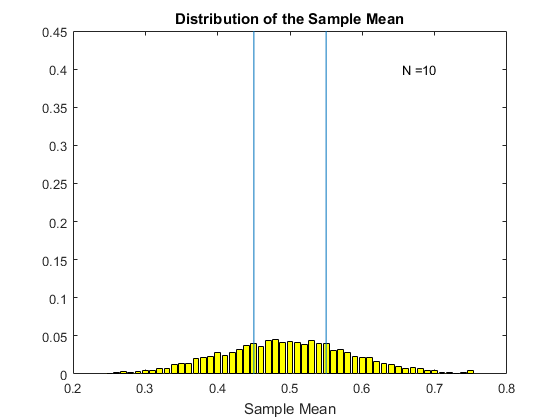
Consider the following gif. Here I have computed the original $X_i$ using a uniform distribution where the random variable takes values from zero to one. I then compute the sample average, and do this 5000 times. Each histogram in the gif is the histogram of these 5000 sample means for various sample sizes. The mean of the sample mean here is 0.5. I choose $\epsilon$ to be 0.05, so the bounds are from 0.45 to 0.55 (we can choose any bounds we want). The bounds are given by the blue vertical lines on the histogram. We see that as we increase the sample size, the distribution of the sample mean becomes more and more concentrated around the mean 0.5. For N=10 we have a lot of sample means outside our bounds. However as we increase the sample size, the distribution gets tighter and tighter (this is the variance decreasing with the sample size) and we have fewer and fewer of the sample mean estimates outside the bounds. Eventually, as N gets large enough, we see that the chance of being outside the bounds dissapears. This is the probability of being outside the bounds going to zero.

When $ P[|\bar{X}-\mu|>\epsilon] \rightarrow 0$ we say that the law of large numbers applies. What it is getting at is that, as in the gif above, that as the sample size gets larger and larger there is a sense in which the estimates of the sample mean become closer and closer to the true mean. In this version of the law of large numbers (known as the weak law) the sense is in terms of the probability of being outside the bounds goes to zero.

The law of large numbers holds for situations where $X_i$ have means (not all random variables have a mean, but most do) and the sample is a random sample. So for all of our problems it holds. It even holds in more complicated sampling schemes where there is some dependence between the observations.

All of this is a bit hand-wavy, but you should get the idea. A formal proof is not all that hard from a math perspective, see here

5.5 The Central Limit Theorem

So in terms of the sampling distribution of the sample mean $\bar{X}$, we know that if the data are drawn from normal distributions then $\bar{X}$ is also normally distributed. But in most studies there is no reason to imagine that the $X_i$ data are normally distributed. In Chapter 4 we saw that any function of a number of random variables had a distribution that depends on the distribution of the random variables in that function. This means that the exact sampling distribution of $\bar{X}$ depends on the exact distribution of the $X_i$. If we knew the distribution of the data, after (sometimes a lot of) hard work we can find the exact distribution for $\bar{X}$. And if we did not know the distribution of $X_i$, we could not even begin. Fortunately though, in large enough samples these problems melt away for sample averages.

In what is one of the more amazing theorems in mathematics and statistics, it turns out that the sampling distribution for $\bar{X}$ when the underlying $X_i$ are a random sample is often very well approximated by a normal distribution. If you wonder what is amazing about it, think of this: because of this theorem in most situations you will encounter instead of having to use a different distribution each time you can use the normal distribution and learn just one set of tricks for the rest of the course.

We are not going to prove this theorem, instead we will state it with the assumptions needed to use it.

Central Limit Theorem. If the data $X_i$, $i=1,...,n$ are from a random sample with mean $\mu$ and variance $\sigma^{2}$, then the sampling distribution of the sample average $\bar{X}$ is approximately equal to a normal distribution with mean $\mu$ and variance $\frac{\sigma^{2}}{n}.$

The result says the following - if we center and standardize our sample averages by the correct mean and correct standard deviation of the mean, then for a large enough sample size $n$ then the distribution of the this centered and standardized sample mean will be approximately equal to the standard normal distribution. We know how to center and standardize, what we want to compute is $$\begin{equation} \frac{\bar{X}-\mu}{\sigma/\sqrt{n}} \end{equation} $$ This statistic will be approximately normally distributed with mean zero and variance equal to one. Now the problem is in the details. First, to do this we need to know the mean $\mu$. We also need to know the variance of $X_i$, i.e. we need to know $\sigma^2$. Finally, the sample size $n$ has to be 'large enough'. We will consider these further on, but for now imagine that we know these values. Then we can use the standard normal distribution to compute approximate probabilities for this statistic. This will turn out to be immenseley helpful.

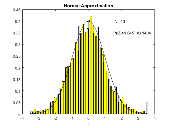
To see this in action, consider the following animation. The underlying $X_i$ used to compute sample means here is the uniform distribution on (0,1), the one we derived in Chapter 3. For each different sample size $N$ shown on the animation, I have computed 5000 times the sample mean from a sample of that size. Then I created a histogram of the distribution of these sample means, which is shown in yellow. The black line is the standard normal distribution. I have also computed the above centered and standardized statistic (called Z in the figure) and calculated the proportion of the 5000 draws that fall either below -1.645 or above 1.645. We know from computing from the standard normal distribution that this should be ten percent if the standard normal is a good approximation (because this is what we would get using the standard normal distribution as an approximation).

What we see in the animation is that the distribution, even for a sample size of 10, is quite similar to the standard normal distribution. The probability of exceeding the stated bound is about fourteen percent, which is not so close to ten percent, but this is a really small sample size. By the time the sample size is 80 observations, we are doing really well and we can see that the approximation is just fine.

Now consider the next animation. In this animation I have done everything as above but now the underlying data are drawn from a chi-squared distribution with degrees of freedom equal to one. This distribution is a very skewed distribution, with a positive skew (not so many small values, lots of large ones). In this case with a sample size of 10 the distribution of the sample means is not close to the normal distribution, indeed the chance of being outside the bounds we calculated should be equal to ten percent is here more than 20 percent. The normal approximation will be very misleading if the sample size is this small. But as the sample size gets larger we see that the normal approximation gets better and better. By $N=160$ it is looking really good, and the chance of being outside the bounds is close to that we expect from the standard normal distribution.

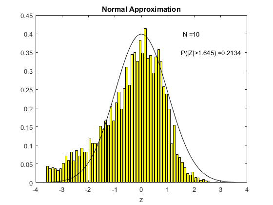
Above I said that the sample size needs to be large enough for the normal approximation to be accurate. What we see in the two animations is that how large the sample size needs to be depends on the distribution of the underlying $X_i$ (this is all that was different between the two animations).

A little aside. Some of you might have seen the situation where we know $X_i$ are normally distribued like in section 5.3, but we do not know the variance and must estimate it. In this case we know the correct distribution of $\bar{X}$, it has a t distribution with $n-1$ degrees of freedom. We however in this course will not discuss this, because it is not a real problem. See here.

5.6 Central Limit Theorem applied to Bernoulli random variables

The central limit theorem is a powerful result that lets us compute probabilities over the sample mean random variable $X_{bar}$ for many different distributions, even when we do not know the exact shape of the distribution. One very useful application, indeed the application for which it was first developed, is when the underlying data is Bermoulli($\pi$) distributed.

The central limit theorem says that if we center and standardize our sample averages by the correct mean and correct standard deviation of the mean, then for a large enough sample size $n$ then the distribution of the this centered and standardized sample mean will be approximately equal to the standard normal distribution when the data are a random sample. For the Bernoulli($\pi$) distribution, suppose We know the value for $p$. Then for $X_i$ we have that the mean is $p$ and the variance is $p (1-p) $. For the general case when we center and standardize, what we want to compute is $$\begin{equation} \frac{\bar{X}-\mu}{\sigma/\sqrt{n}} \end{equation} $$ In the special case of a Bernoulli distribution then what we want to compute is $$\begin{equation} \frac{\bar{X}-p}{\sqrt{p (1-p)/n}} \end{equation} $$ This statistic will be approximately normally distributed with mean zero and variance equal to one. Using this approximation, we can now compute probabilities (or more correctly, approximate probabilities) for sample sizes that get larger than our Binomial tables would allow us.

Example: Consider a polling problem where you will call 1000 people and obtain their opinion on some issue. Our data would be zeros (negative opinion) and ones (positive opinion). Suppose further that we know that the probability that someone is in favor of the proposition is 0.48. This is $\mu$, so when we know both $\mu$ and the sample size we can center and standardize and use the normal distribution to approximate the distribution to compute probabilities.

I want to approximate the probability that when we do this that we obtain a positive opinion more often than a negative opinion. In math I want to compute $P[\bar{X}>0.5]$. We can use the central limit theorem to undertake this calculation. We have $$\begin{equation} \begin{split} P[\bar{X}>0.5] &= P[\frac{\bar{X}-0.48}{\sqrt{0.48 (1-0.48)/1000}}>\frac{0.5-0.48}{\sqrt{0.48 (1-0.48)/1000}}] \\ & \approx P[Z>1.266] \\ & = 0.1028. \end{split} \end{equation} $$ Thus we are able to calculate, very quickly, that the chance of seeing the positives be greater than the negative opinions with a 10 percent chance. This is only approximate since we used the central limit theorem in the second step, and we want to be sure always to keep that in mind. But none-the-less this will be an accurate picture of the probabilities we want to calculate.

The reason we do not have binomial tables up to large numbers is twofold - first, it is really hard to compute the 'n combination s' for large numbers (try it) and second, from the above results we just do not need them. It is easier to use the central limit theorem and approximate. As in the general case, we would like to know how big the sample size needs to be to use this approximation without making big errors. The same points as in the general case apply - when the distribution is skewed then we need larger sample sizes. For the Bernoulli($p$) distribution we have seen that it is symmetric when $p=0.5$, and becomes more and more skewed the closer $p$ becomes to zero or one. So we would be careful if it is close to the boundaries. We also have to be careful when n is not very large - approximation errors can be important. There is a trick to do this well, see here.