
Calculations with the Standard Normal Distribution
In working with the standard normal for doing calculations, we make use of the properties of the standard normal distribution and that probabilities sum to one. The main feature of the standard normal distribution that helps us is that it is symmetric, so all calculations can be made using only one side of the distribution. This is why when you look at normal tables, they only include half the distribution. It may seem a bit archaic today when computers can easily do the computations for you, but working with and understanding these rearrangements of the problem will deepen your ability to understand many other calculations and concepts we deal with.
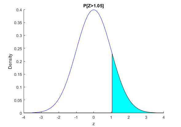
$ P[Z>1.05] $
We first start with a calculation that can be undertaken directly from the usual form of the standard normal distribution, we want to compute $ P[Z>1.05] $. In pictures what we want to do is calculate the shaded area of Figure 1
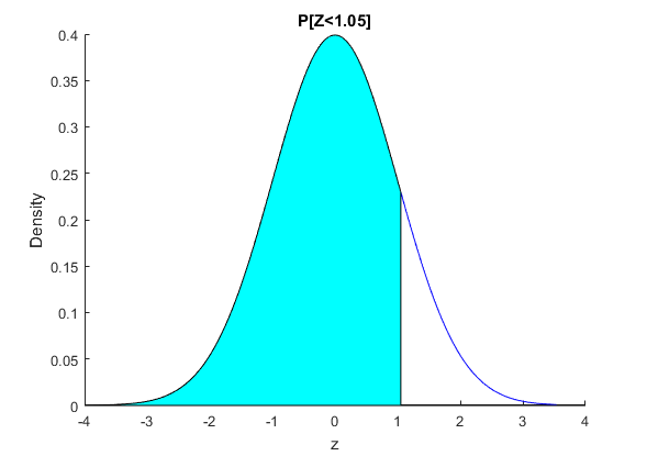
$ P[Z<1.05] $
Now consider computing the $P[Z<1.05].$ In a picture this is Figure 2 below. Comparing FIgure 1 and Figure 2 we see that the sum of these probabilities has to be equal to one - the area under the curve. Hence the events $ (Z>1.05) $ and $(Z<1.05) $ are complements and it must be that $ P[Z<1.05]=1-P[Z>1.05].$ We have turned a problem in the lower tail to one in the upper tail that we can compute from the tables. Hence we conclude that $$\begin{equation} \begin{split} P[Z<1.05] &= 1-P[Z>1.05] \\ &= 1-0.147 \\ &=0.853. \end{split} \end{equation} $$ Notice that we do not have to worry about what is happenning with $P[Z=1.05]$ because for continuous distributions the probability of any point is zero.
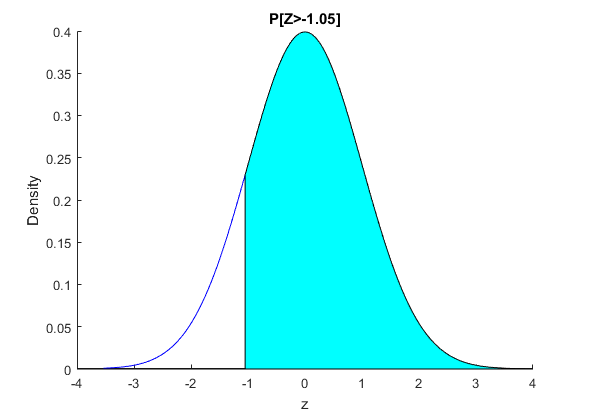
$ P[Z>-1.05] $
Now consider computing the $P[Z>-1.05].$ In pictures this is Figure 3 below. Comparing Figure 2 with Figure 3, it is clear that the shaded areas are the same size. Basically the second problem is the mirror image of the first problem, if we reflect the normal distribution about $z=0.$ Thus by symmetry we know that it must be that $P[Z>-1.05]=P[Z<1.05]=0.853 $
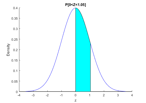
$ P[0<Z<1.05] $
For a slightly more complcated problem, consider computing the $P[0<Z<1.05]$. This is the area shaded in Figure 4. There are a number of ways to compute this, each giving the same answer. The first is to realize that compared to the problem in Figure 2, this is simply removing the area under the curve below zero from Figure 2, i.e. subtracting the $P[Z<0]$ from $P[Z<1.05]$ Since clearly $P[Z<0]=0.5 $ (it is half the area under the curve) then we have that $$ \begin{equation} \begin{split} P[0<Z<1.05] &= P[Z>0] - P[Z>1.05] \\ &= 0.5-0.147 \\ &=0.353. \end{split} \end{equation} $$ Either gets you the same answer.
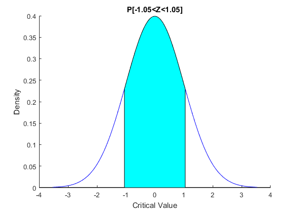
$ P[-1.05<Z<1.05] $
Finally consider computing the $P[-1.05<Z<1.05].$ This is the area shaded in Figure 5. Again, we have multiple ways of computing this. The first is to realize, by symmetry, that this is simply double the area shaded in Figure 4. Hence we have that $$\begin{equation} \begin{split} P[-1.05<Z<1.05] &=2*(P[0<Z<1.05]>0]-P[Z>1.05]) \\ &= 2*(0.5-0.147) \\ &=0.706. \end{split} \end{equation} $$ Alternatively we might also realize that the area shaded in Figure 5 is equivalent to removing twice the area above 1.05 from the entire area under the curve. The area above 1.05 was shown in Figure 1. In this calculation we have $$\begin{equation} \begin{split} P[-1.05<Z<1.05] &=1-2(P[Z>1.05] \\ &= 1-2*(0.147) \\ &=0.706. \end{split} \end{equation} $$ Again, there are many ways to do it, choose the easiest.
All problems using the tables can be handled in this manner.
Copyright © Graham Elliott
Distributed By Themewagon