
Chapter 3 Worked Examples
We go through a simple example of a discrete random variable and a continuous random variable to show how the calculations work.
Discrete RV example
Consider the distribution in the following table:
| $X$ | $P(X=x)$ |
|---|---|
| 1 | $ \frac{4}{10}$ |
| 2 | $ \frac{3}{10}$ |
| 3 | $ \frac{2}{10}$ |
| 4 | $ \frac{1}{10}$ |
In a graph it is simply
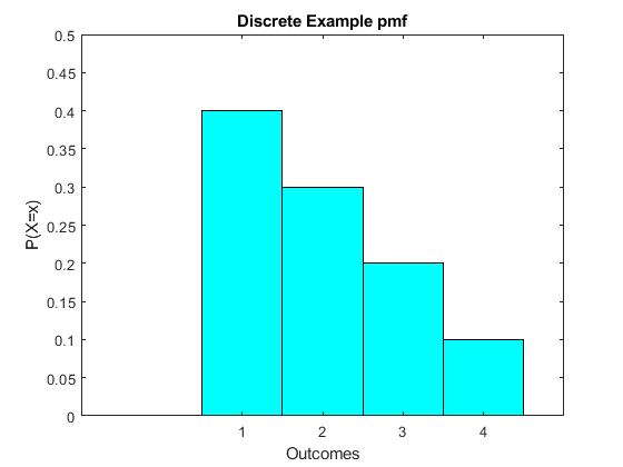
We can easily compute probabilities of various events. For example if we want $$ P(X>2) = P(X=3) + P(X=4) = 0.2 + 0.1 = 0.3. $$ What you should realize is that this is the area under the pmf for $X=3$ and $X=4$.
Looking at the probability mass function, we can guess the mean as the balancing point. Clearly the weight is towards lower values, seems like it is above 1 but at a maximum 2.
Instead of eyeballing the mean (which we should do as a check on the math) we can simply use our formula to compute it. Recall that $$ EX = \mu = \sum_{x} x P(X=x) $$ so we have $$\mu = 1*0.4 + 2*0.3 + 3*0.2 + 4*0.1 = 0.4+0.6+0.6+0.4 =2. $$ So the mean is two.
The variance we cannot eyeball, but we can calculate it using our formula. Recall the general formula for a discrete random variable is $$ Var(X) = \sigma^2 = \sum_{x} (x-\mu)^2 P(X=x) $$ so we have $$ \sigma^2 = (1-2)^2*0.4 + (2-2)^2*0.3 + (3-2)^2*0.2 + (4-2)^2*0.1 = 1. $$ So the variance is equal to one. We have not learned why we care about the variance but it will become clear later in the course.
Continuous RV example
Consider the probability distribution function $$ p(x) = x + \frac{1}{2} $$ where $0 \le x \le 1$.
The pdf can be visualized easily, we have the distribution in the following figure.
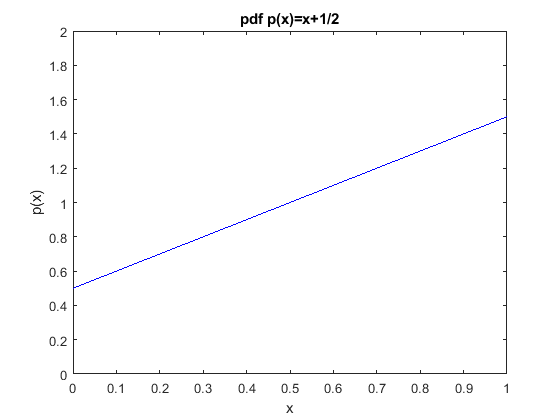
First, we should verify that it really is a pdf. For this we need that it is always nonnegative and that it integrates to one (because probabilities are areas under the curve, and probabilities of everything must be one). It is fairly obvious from the figure that the curve is non-negative. But also from the formula, we see at its lowest point it is one half. In terms of integrating to one, we can fairly easily determine that it does, either from some quick calculations of squares and triangles from the figure or just directly integrating the equation mathematically. First, do the math. We have that $$\begin{equation} \begin{split} P[0 \le X \le 1] &= \int_0^1 (x + \frac{1}{2})dx \\ &= \left [\frac{x^2}{2} \right]_0^1 + \frac{1}{2} \left[x \right]_0^1 \\ &= \frac{1}{2} + \frac{1}{2} = 1. \end{split} \end{equation} $$ So yes the pdf is a pdf. To do using rectangles and triangles look at the figure. The area under the curve is the rectangle from zero to one equal to a height of one half (so has area one half) plus the triangle above it. The triangle is half of the rectangle with height one and width one, so has area one half. Add them together and you get one.
We can work out other probabilities in the same way. For example to work out the $P[X<\frac{1}{4}]$, we have $$\begin{equation} \begin{split} P \left[0 \le X \le \frac{1}{4} \right] &= \int_0^{\frac{1}{4}} (x + \frac{1}{2})dx \\ &= \left[ \frac{x^2}{2} \right]_0^{\frac{1}{4}} + \frac{1}{2} \left[x \right]_0^{\frac{1}{4}} \\ &= \frac{1}{32} + \frac{1}{8} = \frac{5}{32}. \end{split} \end{equation} $$ This is the area under the figure from zero to one quarter. All probabilities are worked out as areas under the curve over the relevant range you are looking at.
To compute the mean of this, we can first consider the balancing point. Obviously it is above one half, because if it were flat it would balance at one half but we have more mass to the right so it is going to be higher. Beyond that, it is hard to say how far. So to the math. We have $$\begin{equation} \begin{split} EX &= \int_0^1 x (x + \frac{1}{2})dx \\ &= \left [\frac{x^3}{3} \right]_0^1 + \frac{1}{2} \left[\frac{x^2}{2} \right]_0^1 \\ &= \frac{1}{3} + \frac{1}{4} = \frac{7}{12}. \end{split} \end{equation} $$ So yes, a bit above one half as we visualized.
This seems like tedious math, mainly because it is math and it is often tedious. However there is a point. We will see the point in Chapter 5 onward, where the mean relates to our theories. It will turn out that we also need the variance, which is even more tedious (and still math). I will leave that to you for now, but it is just integrating away.
Copyright © Graham Elliott
Distributed By Themewagon